
Statistics
- Univariate Analysis – measuring one thing, like just HR
- Multivariate Analysis – measuring more than one variable
- Bivariate Analysis – measuring exactly two variables (x and y) in order to try to understand a relationship between the variables.
- Coefficient of correlation (r)
- Has a range of [-1,1]
- Negative r value indicates a negative correlation
- As x increases, y decreases
- If r = 0, slope of line of best fit is likely going to be 0
- Coefficient of determination (r^2)
- Has a range of [0,1]
- This is only r^2 in simple linear regression (bivariate situation)
- Equation of Best Fit Line
- The slope of a line of best fit determines the change in incrementing an item
- For example, if you’re plotting Runs/G vs. Win %, one more run give you an increase in likelihood of winning equal to the slope of that line of best fit
- Run differential has a very strong R^2
- Improving run differential by 1 R/G, Win % increases 10%
- Cause and Effect
- We don’t really know if run differential causes an increase in win percentage
- We just know that there is a relationship
- A confounding variable can cause deceiving relationships. For example, plotting drowning against ice cream consumption will yield a positive relationship. But the weather/temperature is a confounding variable that affect both.
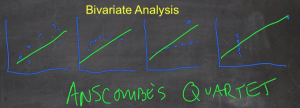
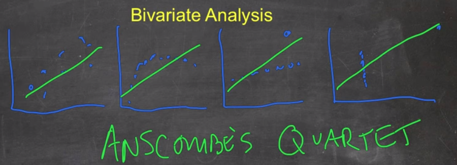
- Lines of best fit
- Can be deceptive.
- R and Line of Best Fit can be the same for various sets of data
- Anscombe’s Quartet – always look at your data, your scatter plots. Make sure you look at the nature of the data.
Sabermetrics
Offensive Eras
- Different eras and run scoring environments in the history of baseball
- Run scoring environment in 1800s was very unstable, large swings, maybe sample size issues? Or fundamental?
- Many rule changes in 1800s
- 1877 eliminated fair-foul hit (ball hit in fair territory then went foul before first base)
- 1880 reduction in number of balls required for a walk from 9 to 8. Continued to drop until 1889 (4).
- 1883 pitchers had to deliver pitch below the waist prior to this. Changed to shoulder high.
- 1887 batter could tell pitcher if they wanted high strike or low strike. Changed strike zone to be similar to now.
- 1893 moved mound to current distance.
- 1898 balk rule. Started tracking stolen bases.
- 1901 marks beginning of modern era.
- 1900 – 1920Deadball Era, inconsistent manufacturing, would use the same ball during the game, trick pitches (spitballs, etc.)
- 1910 – 1915 Emery Ball (scuffing)
- 1920 – 1940 Live Ball Era, Babe Ruth comes along, death of Ray Chapman who died on field and didn’t even see the ball. Led to replacing of baseballs. Consistent manufacturing of balls.
- AL has higher run scoring
- 1940 – 1945 War Era
- 1941 – 1960 Integration Era. Included War Era rosters missing many good players. 1947 Jackie Robinson.
- 1960 – Today
- Expansion of 16 teams to 30 today
- AL adopts DH
- 1969 shrunk strike zone, lowered top and raised the bottom. And lowered pitcher mound.
- Free agency
- Mid 1990s – 2010 Long Ball, Steroid era
- Not a noticeable run scoring difference between AL and NL until 1979, we see a split where AL begins to score more. DH rule was adopted in 1973.
- Home runs/G generally increase steadily from 1900 – 2010
- Stolen bases declined greatly from 1900 – 1930. Then there are waves of increasing and decreasing.
- Sacrifice hits have declined steadily.
- K/9 has increased from about 3-4/G to over 7.5/G now
Relationship Between Runs and Wins
- Alan Roth and Branch Rickey were first to look at this relationship more closely
- RD = R – RA (run differential = runs scored – runs allowed)
- Can pull run differential information from the Teams table in the Lahman database
- Using just R and RA doesn’t measure perfectly because there are seasons with different years. Need to convert to R/G and RA/G
- Few teams ever had more than +2 R/G differential
- +1 R/G differential gets you around .600 WPct
- Negative relationship – when increasing one variable causes the other to decrease, example is RA/G on WPct
- Positive relationship – when increasing one variable causes the other to increase, example is R/G on WPct
- Bill James’ Pythagorean Theorem = R^2/(R^2+RA^2)
- If you change exponent to 1.83 (instead of 2), it becomes a bit more accurate
- 1954 started tracking sacrifice flies
- 1955 started tracking intentional walks
- 1955 forward is a nice choice for starting your analysis because they were then tracking all the stats commonly used then.
- Kross estimator was most accurate from 1901 – current. Pythagorean 1.83 has lowest average difference for 1955 – current.
- If we can determine what a run scored is worth in terms of wins (or a run against prevented), we can start to determine the value of specific players.
- These measures of winning percentage use Runs as an input. So if we can estimate the amount of runs a player contributes or saves, we can estimate the number of wins that will contribute to the team.
- Approximately 10 runs = 1 Win
Technology
Joins
- Each table has a unique key that represent an index or a unique identifying number for each record
- A join takes information from two different tables
- Always try to join on fields that are indexed/primary keys
- SELECT xxxxx
FROM yyyyy y
JOIN zzzzzz z
ON y.ID = z.ID - SELECT xxxxx
FROM yyyyy y
JOIN zzzzz z
ON (y.ID = z.ID
AND y.ID2 = z.ID2)
- If your SQL processing is taking a long time, it’s probably because you’re not using primary keys
- Do the GROUPBY after the JOINs, putting it before can really slow things down
Inner Join
- When you specify JOIN, this is the default Join type
- When doing a JOIN, the left table in the Venn diagram is the table specified in the FROM clause, the right table in the Venn diagram is the table specified in the JOIN clause
- The INNER JOIN is the overlap. Only items that appear in both tables.
Left JOIN
- All items from the left table in the Venn diagram are included, even if they don’t have a match in the right table
Right Join
- All items from the right table in the Venn diagram even if they don’t have a match in the left table
SELECT
- Can concatenate two fields into one field
- SELECT CONCAT(nameFirst, ” “, nameLast) AS PlayerName
Table Aliasing
- SELECT blah blah
FROM Batting b
JOIN Master m
ON b.playerID = m.playerID - This “Batting b” is shortening the table name to just b for this query
Nested Selects
Select w.yearID, AVG(ABS(w.Error)) AS AverageError
From(
SELECT teamID, yearID, W,
G*(R^2)/(R^2 + RA^2) AS predictedW,
(G*(R^2)/(R^2+RA^2)-W) AS Error
FROM Teams
WHERE yearID >= 1955
) w
GROUP BY w.yearID
History
FC Lane
- Writer about baseball, over 1,000 pieces
- Wrote a lot of biographical pieces
- Influential book called Batting
- “BA worse than worthless”
- Studied how runs are scored
- “Why would a system that placed nickels, dimes, and quarters on the same basis be much of a system whereby to compute a man’s resources”. BA equally values all hit types.
- Studied the value of each hit type and approximately how many runs it was worth