How To Add Positional Ranking To Your Spreadsheet

I just came across an interesting use of an Excel formula that will let you easily determine what a player’s ranking is at their given position (1B-1, 1B-2, 1B-3, etc.).

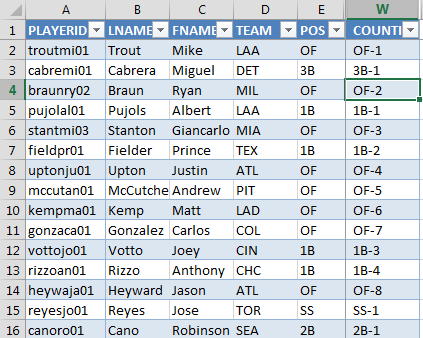
Here’s an explanation that might show what I’m talking about.  You’re scrolling through your huge list of ranked hitters (see image below).  You have them sorted by Total Standings Gain Points (column V) in descending order.

You see Edwin Encarnacion’s name pop up in row #38.  You know he’s a first basemen, and you can pretty easily determine that he must be the #37th ranked player (by showing up on row 38).  But now you want to know where he ranks amongst only other first basemen.

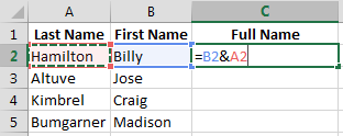
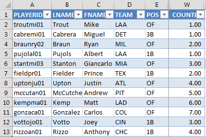
In this post I’ll show you a formula we can use to get our spreadsheet to look like this (look at column W):

I’m a Moron

I got nearly to the end of this post when I started to think it was weird that Encarnacion was ranked #37, Starlin Castro #32, and Paul Goldschmidt #21. Turns out I used a rankings file from the 2013 preseason for all the screenshots…

I decided against starting over because it’s not the player names that are important, we’re mostly looking at a new formula. And I found it pretty interesting and thought provoking to look at these old lists and see names like Nori Aoki and B.J. Upton so high.

Excel Formulas Used In This Post

Using the “&” to Build Text

As you can see from the image above, we’re trying to take each player’s position (e.g. “1B”) and then add a dash and then the player’s positional ranking (e.g. “1B-8” for Encarnacion).

You can use the ampersand (would you know what that was called without “Wheel of Fortune”?), in an Excel formula to add text from different columns.

A real practical application of this is to build a player’s full name (e.g Billy Hamilton) from their first name and last names being in separate columns.  Here’s an example:

I did leave something important out of this formula.  Look what happens: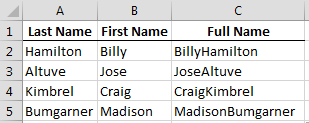

Just appending the two fields together leaves out a space between the first and last name.  So to revise the formula, we can add a space between the names like this: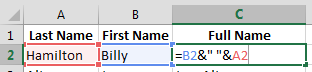

We’re now putting three pieces of information together.  Cell B2 plus a space (” “) plus A2.  And you can continue adding on information with more “&” symbols.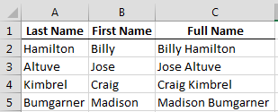

You may be familiar with Excel’s CONCATENATE function which does the same thing, but I just find this easier to use.

COUNTIF

The COUNTIF formula will count the number of cells in a specific column (or other range) that meet a specified condition.

In plain English, our goal is to have Excel count the number players that have the position of first basemen (1B) in column E.

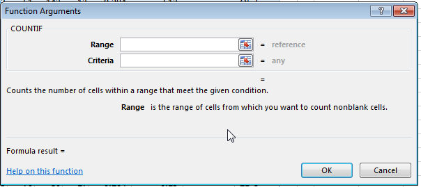
As you can see from the function wizard above, this formula requires two inputs:

COUNTIF( Range , Criteria )

1. Range – This is the block, column, or area of cells we want to count from.  “Excel, look in Column E and count the cells that meet this condition I’m about to tell you about in bullet #2.”
2. Criteria – This is what we are evaluating the cells for.  “Count the cells in Column E that show ‘1B’ as the position.”

More About The RANGE We Want In The COUNTIF Formula

I simplified things above.  Thinking more closely about this, we don’t really want to count the total number of “1B” in Column E.  For Albert Pujols, the very first “1B” in the column, we only want him counted.  For Prince Fielder, the second “1B”, we want only him and Pujols counted.  For Paul Goldschmidt, the seventh “1B”, we want him and all those before him.  And so on.

To accomplish this we need the range of cells we’re looking in to change as we move down the player list.

Here’s a graphic of the range we want for Pujols.  Check out the highlighted cells.  We would want to count the number of 1B in cells E2 through E5.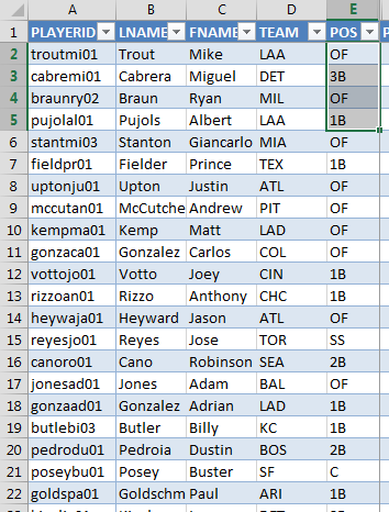

And here’s one for the range we want for Paul Goldschmidt.  We would want to count from E2 to E22.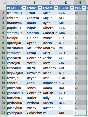

So the range the we want needs to be able to expand as the formula moves down the column.  The way to do this in Excel is with the concept of absolute and relative cell references.

We want the “E2” part of the range to be frozen  in place.  But we want the second part, “E5” (in “E2:E5”) or “E22” (in “E2:E22”) to move.

To do this, we will specify to Excel that the first cell in our range is “absolute” and that the second cell is “relative”.

We do this by putting a dollar sign in front of the row number of the absolute cell.  You can put the dollar sign in front of the column if you don’t want the column to change as the formula moves.

E$2:E5

As the formula is moved down the column, the dollar sign tells Excel not to move the E2 reference.

Enough Concepts.  What’s the Formula?

Step	Description
1.	I’m going to build this formula in pieces.  First, create a new column to hold “POS RNK”. And we’ll start with just the COUNTIF formula for now.
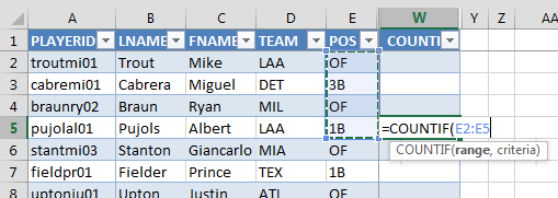
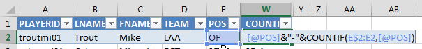
2.	I think it will be helpful to start the formula with about the fourth or fifth player in the sheet and not the first player. In my example, I typed “=COUNTIF(” in cell W5.  I then used my mouse to select from cell E2 to E5 (because my position is in column E).
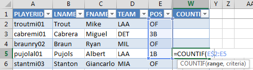
3.	Now place your mouse cursor and click in front of the “2” in the formula we’ve started.  Then type the “$”. That finishes the “Range” part of the formula, and now we can move to the “Criteria”.
4.	Type a comma after the “E$2:E5” argument, and then click on cell E5.  Then close the parentheses on the formula.  The criteria is the position of any given player.  For Paul Goldschmidt, we want to count him and also the number of 1B above him in the rankings so we can determine where he falls in the rankings. If you’re using an Excel “Table”, like I frequently use on the site, the formula probably came out as something like this: If not, it probably came out with a reference to cell “E5” like this:They both work.  Hit enter to save the formula.  You should see the counting take place. Spot check that it’s working by picking a player and a position to count.  In my example, I can see that Pujols is the first 1B, Fielder is second, Votto is third, and Rizzo is fourth.
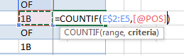
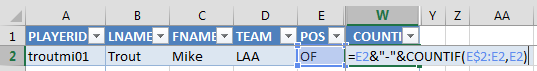
5.	Now we can add in the text part of the positional rankings to turn each of these into the “1B-1”, “1B-2”, and “1B-3” format. Be careful to note that now I’ve switched up to editing the formula in cell W2 (for Mike Trout).   Click your mouse between the equals sign and the “COUNTIF” part of the existing formula.  Our goal is to add the “1B-” part of the formula using the ampersand to build the text. 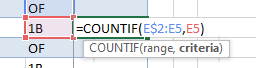My final formula if you are using an Excel Table is: =[@POS]&”-“&COUNTIF(E$2:E2,[@POS]) If you’re not using Table References: =E2&”-“&COUNTIF(E$2:E2,E2) Hit Enter.  We’re done!

Have Other Questions About How To Do Things Like This?

If you have questions about making an awesome rankings or draft spreadsheet, let me know.  You can comment below or e-mail me at smartfantasybaseball at gmail dot com.

If you’re interested in similar articles in the future, following the site on Twitter or registering as an Insider are the best ways to keep up-to-date.