In the middle of the distribution the mean, median, and mode are the same
You can try to apply the normal distribution to baseball talent
But we usually measure outcomes, not talent
Be clear about what you’re doing
Bill James first to write about “replacement level” instead of just average (1984 abstract, 1985 abstract)
Earlier writers argued for using average as the comparison point
James also argues that baseball talent is not normally distributed, it’s skewed.
Keith Woolner has a great explanation of replacement level in 2002 Baseball Prospectus Annual
Some people talk about replacement level as “the bench player” while others talk about the “zero cost option” (free agents, 26th man, etc.). Make sure you understand
Best method of using replacement level is to do it for each position
Console is on the left of the window and is where the coding takes place
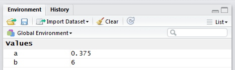
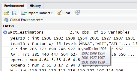
Environment tab is on the top right and displays your variables while moving through the code
History tab is also on the top right. The “To Source” button sends selected code to a text editor window that can be used to save code for later use.
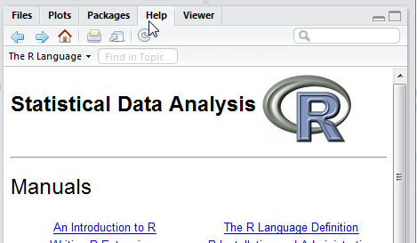
Help is on the bottom right and is very good, detailed
Set variables as you would in traditional programming (e.g. a = 2 + 4, a =6)
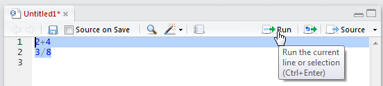
You can highlight code and then use the “Run” command in the Source window, then just the highlighted code gets run
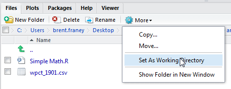
Before you start doing work you need to “Set a Working Directory”
R Tips and Tricks
CTRL + L clears all information in the Console
Up and Down arrow keys allow you to cycle through the different commands you have already typed into the Console, an easy way to rerun a command
R Variable TYpes
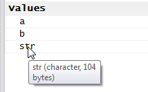
Can hover over variables in the “Environment” tab to see what type of variable you have (string, number, etc.)
Numeric
String
Logical (Boolean, True/False)
R Data Frames
Similar to a spreadsheet or database
Multiple columns, each column can be of different data type
R Console Commands
summar(dataset_name) – returns min, max, median, mean, 1st quartile, 3rd quartile for each field in the dataset
view(dataset_name) – loads the data set into a table view
mode(variable_name) – returns the data type (str, num, bool)
plot(dataset$fieldname_for_x_axis,dataset$fieldname_for_y_axis,xlab=”x axis label”,ylab=”y axis label”, pch = “plot data point type e.g. diamond, circle, etc.”, col=”color of plot data points”) – scatter plot of one field on the x axis and one field on the y axis
sqrt(dataset_name$fieldname) – square root
head(dataset_name) – gives top several records at the top of the dataset
tail(dataset_name) – bottom six records in the dataset
HISTORY
Allan Roth
First full-time statistician employee for an MLB club
Suggested tracking all kind of split information (day/night, left/right, counts, batted ball location, etc.)
A huge data collection driver
In 1950 Branch Rickey went to PIT, but Roth stayed with Dodgers.
The 1954 LIFE article from Rickey and Roth was groundbreaking
First time run differential was used to analyze success
They modelled offense and defense using the formulas they built
O – D = G
Offense – Defense = Games Behind
Offense = OBP + ISO + “Clutch”
Defense = OPP BA + WALK/HBP + “Pitching Clutch” – Strike Outs – Fielding
We use cookies to ensure that we give you the best experience on our website. If you continue to use this site we will assume that you are happy with it.