An Important Lesson and How to Resolve VLOOKUP Errors

Let me come clean. I screwed up. And it likely will cause you to see errors in your spreadsheets. That’s the whole reason for this post.

Having trouble with VLOOKUP error messages? This post should help.

What Happened?

While this post is going to address a very important topic (resolving VLOOKUP errors), there wasn’t much of a need for this until I came up with a new format for the Player ID Map. The intent was to make the Player ID Map easily updatable. I hate having to lookup the IDs, birth dates, and handedness of all the new players.

And it’s always bothered me that there was no easy way for you to get updated Player ID information.

Let’s be honest. It’s a pain in the ass. Especially this time of year when players are switching teams every day and minor league players we haven’t had to deal with in the past are now projected to reach the big leagues this season. It’s tedious to keep teams up-to-date and to add these new players.

I needed to find a way to improve this process and to make everyone’s lives a little easier.

The Solution

The solution was to make the Player ID Map available in an online CSV file. One you connect that online file to your Excel spreadsheet, you simply have to right-click on the Player ID Map and hit “Refresh”. You will instantly get any update I’ve made.

Sounds amazing, right?

Major leaguers  have a purely numeric Fangraphs ID while minor leaguers have text in their ID.
Major leaguers have a purely numeric ID while minor leaguers have text in their ID.

The Problem

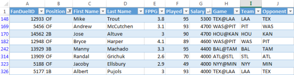
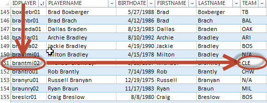
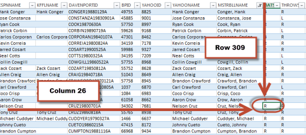
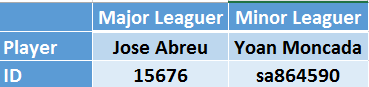
The fly in the ointment happens to be the way Fangraphs structures their player IDs. Major leaguers, like Jose Abreu, have a purely numeric ID. Whereas minor leaguers that have not reach the big leagues, like Yoan Moncada, have the text “sa” in front of a string of numbers.

The unintended consequence of importing the Player ID Map file is that because some IDs contain text, Excel will treat the ENTIRE imported column as text.

The problem is that reports you download from Fangraphs and then open in Excel treat the player ID column as numeric values.

Warning… It’s About to Get Technical

If you’re fine with the old Player ID Map and the fact that it doesn’t get updated very often, you don’t have to use the new one. The old one can be downloaded here and will still be updated periodically. You can stop reading this post and save yourself some sanity.

But if a little complication doesn’t scare you off and you see the value in being able to refresh the Player ID Map and get regular updates… Keep reading.

Text and Numbers Are Treated Differently

Excel and most other computer applications treat text and numbers differently. And this is a common problem with VLOOKUPS. So the number “15676” is not the same as a text string of “15676”. So in our VLOOKUPS, we need to make sure we are comparing numbers to numbers and text to text.

Consider the Error Message

The first step in resolving a VLOOKUP problem is to understand the error message you’re seeing.

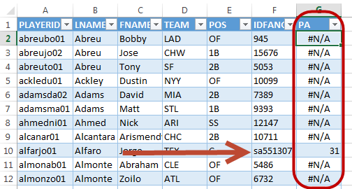
The “#N/A” error is the most common VLOOKUP error. And it essentially means that a match was not found during the lookup.

There are two main reasons a match would not be found:

  1. The item (player ID) doesn’t exist where you told Excel to look for it
  2. Or you told Excel to look for the wrong data type (look for a text value in a list of numbers, or vice versa)

These are the downloaded Steamer Projections. Abreu's ID is the there. It's in the first column. Why isn't the VLOOKUP finding this???
Abreu’s ID is the there. It’s in the first column. Why isn’t the VLOOKUP finding this???

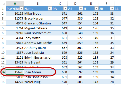
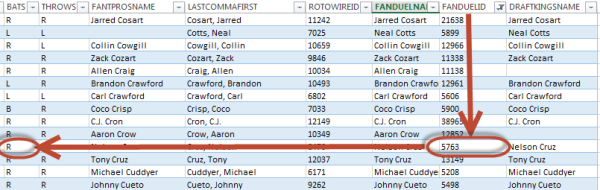
You can easily test the first error by manually performing the search yourself. Let’s walk through a hypothetical example with Jose Abreu. He’s a well known player. He’ll surely be in the Steamer projections I’ve downloaded.

I see from the data that Abreu’s Fangraphs ID is 15676. If I trace that through into the Steamer Hitter projections, I am able to locate Abreu. So why isn’t the VLOOKUP finding the same match?

Continue reading “An Important Lesson and How to Resolve VLOOKUP Errors”

How to Add Batter and Pitcher Handedness to your Daily Fantasy Baseball Spreadsheets

In this post I’ll show you how to add batter and pitcher handedness to your spreadsheets. To do this, we’ll have to learn two new Excel formulas we have not tackled yet.

I’ve avoided doing this for a long time… But there’s just no way around it now. It’s time to say goodbye to relying exclusively on VLOOKUP. Let’s put on our big boy pants and tackle VLOOKUP’s more flexible and powerful counterpart… INDEX and MATCH.

Sometimes VLOOKUP Can’t Get the Job Done

Take this scenario. You’ve started to build a DFS spreadsheet and you’ve imported FanDuel player salaries from a CSV file. Now you want to add player handedness (Lefty/Righty) as a column to your spreadsheet.

FanDuel Player Salaries Excel CSV
FanDuel Salary Information

You are also aware of the Player ID Map and know that it’s an easy way to get handedness information on players.

Batter_Pitcher_Handedness-e1438976169811
The Player ID Map contains information for batter and pitcher handedness, date of birth, team, position, and many player ID and naming systems.

You look at this data above and you think, “No problem!”. FanDuel ID is in both sets of data. How hard could this be? A simple VLOOKUP and we’re done.

But you quickly realize things are not that easy. You see, the VLOOKUP has a very restrictive assumption. If you are doing a VLOOKUP from the salary information into the Player ID Map, the Excel function assumes that “FanDuelID” will be the FIRST column in the Player ID Map.

And that’s NOT the case.

Let’s look at an example VLOOKUP formula:

=VLOOKUP([@FanDuelID],PLAYERIDMAP,10,FALSE)

In this formula we’ve told Excel to go look for the “FanDuelID” column in the “PLAYERIDMAP” table and give us back the value in the 10th column.

But “FanDuelID” is not the first column of the PLAYERIDMAP. It’s the 33rd (wow… the Player ID Map is getting to be quite large). So VLOOKUP will not work.

Other Weaknesses of VLOOKUP

Not only is assuming the data you want to match is in the first column awfully restrictive, if you think about it, VLOOKUP also ties you to a left-to-right lookup. For example, if you’re trying to use Excel to VLOOKUP which team Michael Brantley plays for, his player ID must be in the first column of your data set and you are then forced in to looking only to the right.VLOOKUP_LEFT_TO_RIGHT

We want a formula that will allow our lookup to be in any column and then to look to the left! For example, go find Nelson Cruz’s FanDuelID and then look to the left a few columns and give me the side of the plate he bats from.INDEX_MATCH_LOOK_LEFT

=VLOOKUP([@FanDuelID],PLAYERIDMAP,10,FALSE)

Going back to this example formula right above, the hard coding of a “10” in the formula to return the information in the 10th column is a flimsy approach, but that’s how many people are taught to write VLOOKUP formulas.

The flimsiness comes in if you decide to insert a column somewhere in the PLAYERIDMAP. If column 10 becomes column 11, Excel will not adjust its formula accordingly. Because you are likely building a spreadsheet that you’ll use all throughout the season, it seems highly likely you’ll want to add a new piece of information to your analysis. That inevitably means adding columns to bring that new information in. You don’t want to have to hunt through your formulas to figure out what the new column number in your VLOOKUP needs to be.

Enter “INDEX” and “MATCH”

That’s right. To defeat the almighty VLOOKUP formula, we need to combine the powers of two functions (that last sentence just made me think of this). Let’s take a look.

INDEX

When I’m using a function I’m unfamiliar with, I will add it through the “Insert Function” button. I like doing this because Excel will then give you a search menu to find a formula. And after locating your function you’ll get a helpful wizard that breaks down all the inputs it needs. INSERT_FUNCTION

If you follow that approach to add the INDEX function, you’ll soon realize there are two versions of it.

Excel Index formula has two versions.

I always use the first version, which allows us to locate a cell anywhere within a block of data and return the value from that cell. This function uses the following inputs:

INDEX(Array, Row_num, Column_num)
  1. Array – The range of cells you are searching for a value in. This could be a table or a block of cells.
  2. Row_num – The row within that array that the value is in. This should be a number representing the row.
  3. Column_num – The column within the array that the value is in. Again, this should be a number representing the column (not the letter representation of the column).

It may help to see a visual representation of the function. Assume we’re trying to find Nelson Cruz’s batting handedness. If we tell the index function to look in the PLAYERIDMAP (the “array”), in row 309 (“row_num”), and column 26 (column_num), it would return “R”.

Index Excel formula image example.

We know the array to look in. And we can easily determine the column we want to look in. The challenge we now face is how to determine the row to look in… How do we easily determine that Nelson Cruz is listed on row 309. That’s where the “MATCH” function can help us.

MATCH

The MATCH function will look for a specific value in a range of cells. The function will return a number representing where the matched item falls in the list.

Translating that into English, a realistic use for the function is to look in an entire column for a match. The function will start at the top of the column and proceed down until it locates the desired value. The function then returns where the item falls in the list, which happens to be the row the item is in.

The function uses these inputs:

MATCH(lookup_value, lookup_array, [match_type])
  1. Lookup_value – This is the value you are hoping to match in the array (or column). For us, this will usually be a Player ID of some sort.
  2. Lookup_array – This is the area you are searching for the match within. When using the MATCH function with the INDEX function, this will usually be a column of data.
  3. Match_type – This is an optional input telling Excel some more details about the kind of match you are looking for. You can enter a 1, 0, or -1. Entering a 1 or -1 are forms of approximate matches and are useful if you are looking up numeric values. But we are typically looking to match strings (I consider a Player ID made up of all numbers to still be a string) of text.

    This means we want exact matches only. Accordingly, I always use a 0 for this argument (even though it’s optional, leaving it blank tells Excel an approximate match is acceptable).

MATCH_FUNCTION

Combining INDEX and MATCH

As I alluded to before, the power of these two formulas comes when you combine (or nest) them together. Recall that the INDEX function looks like this:

INDEX(Array, Row_num, Column_num)

If we drop the MATCH function in place of the “Row_num” argument:

INDEX(Array, MATCH(lookup_value, lookup_array, [match_type]), Column_num)

We now have a formula that is more flexible and powerful than a VLOOKUP! The combination of INDEX and MATCH can look for a value anywhere in a table of data and we are no longer tied to the first column and a right-only lookup.

Step-by-Step Instructions

Continue reading “How to Add Batter and Pitcher Handedness to your Daily Fantasy Baseball Spreadsheets”