Welcome to the first part of a series in which we’ll go step-by-step through the process of using Microsoft Excel to calculate your own rankings for a fantasy baseball points league (as opposed to rotisserie or head-to-head rotisserie).
Whether you’re in a standard points league at a major site like ESPN or a more advanced Ottoneu league at Fangraphs, this process will help you develop customized rankings for your league. These instructions can be used for a season-long points league or a weekly head-to-head points league.
If you’re looking for info on how to rank players for a roto league, look here.
I recommend going through all the parts of the series in order. If you missed an earlier part of this series, you can find it here:
ABOUT THESE INSTRUCTIONS
- The projections used in this series are the Steamer 2015 preseason projections from Fangraphs. If you see projections that you disagree with or that appear unusual, it’s likely because I began writing this series in December 2014, still early in the off-season.
- For optimal results, you will want to be on Excel 2007 or higher. Some of the features used were not in existence in older versions.
- I use Excel 2013 for the screenshots included in the instructions. There may be some subtle differences between Excel 2007, 2010, and 2013.
- I can’t guarantee that all of formulas used in this series will work in Excel for Mac computers. I apologize for this. I don’t understand why Excel operates differently and has different features on different platforms.
IN PART 5
In this part of the series we will use the named cells created in Part 2 along with our projection information on the “Hitter Ranks” and “Pitcher Ranks” sheets to calculate total projected points for each hitter and pitcher.
Please note that this series has been adapted into a nine-part book that also shows you how to convert points over replacement into dollar values and how to calculate in-draft inflation. Click here if you’re interested in reading more about the conversion to dollar values.
EXCEL FUNCTIONS AND FORMULAS IN THIS POST
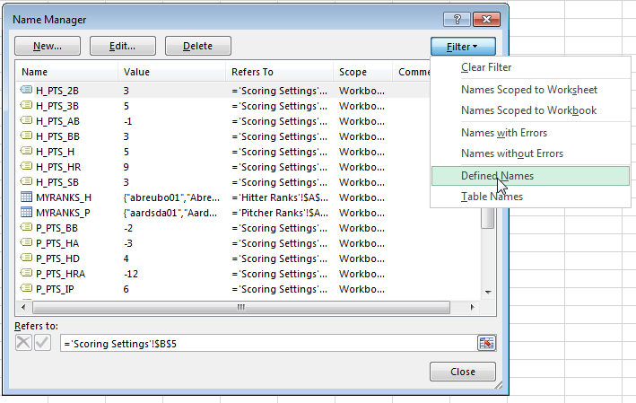
We’ll just be doing some basic addition and multiplication. We won’t be adding in any new features, but we will be doing this basic math using the named cells for your league’s scoring settings that we created in earlier parts of the series. 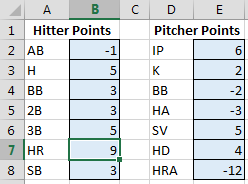 To refresh your memory and to see the complete list of named cells, access the “Formulas” tab of the Ribbon and then click the “Name Manager” button.
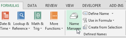
The list will display all named cells/ranges and named tables. To view only named cells, click on the “Filter” drop down menu and choose “Defined Names”.