In this post I’m going to put a slight twist on the Draft Kings CSV salary file import we discussed recently and show you how to import the data into an “Excel table” (or sometimes referred to as an Excel structured reference).
If you’ve followed any of my previous “how to” sets, you know I’m a big proponent of using these Excel tables. They give a number of benefits:
- Efficiency – When you add a formula to a cell, Excel automatically copies that same formula to all other rows in the table. No more copying and pasting and scrolling around to copy your formulas.
- Consistency – Reduces the likelihood of an error in your spreadsheet by making sure formulas in a column are identical.
- Easier to Build Formulas – Your table becomes part of Excel’s reference system giving you useful type ahead features
- More Reliable Formulas – Because of the naming and reference system, formulas can better adjust when rows/columns are added or deleted. Ever had a VLOOKUP formula fall apart after you added a column to your spreadsheet? Or how do you think your spreadsheet will respond when you import a large list of players for a big slate of games and the next day you play a small slate of afternoon games? Setting the range of salaries as an Excel table allow formulas to adjust automatically.
- Meaningful Formulas– Structured reference formulas inherently have more meaning to them than standard formulas not using structured references. Look at these two examples…
Traditional Excel Formula
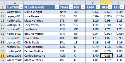
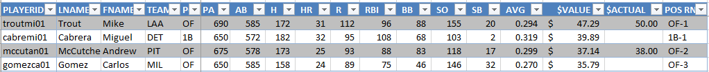
=VLOOKUP(A3,PLAYERIDMAP!$A$1:$AH$1502,4,FALSE)Structured Reference Excel Formula
=VLOOKUP([@PLAYERID],PLAYERIDMAP,COLUMN(PLAYERIDMAP[FIRSTNAME]),FALSE)While the first formula is shorter in length, it’s also shorter on meaning. You can’t look at the formula and easily determine its purpose. You can easily look at the second formula to see it’s trying to locate the PLAYERID in the PLAYERIDMAP table and return the FIRSTNAME of the player.
I think this is a HUGE benefit…
Is This Really Necessary?
Necessary? Probably not. An improvement? I think so. Since discovering Excel’s structured reference system, I’ve been using it on all my spreadsheets. I was excited to find a way to do this while importing data from an outside source. I didn’t know it was possible… I just wish we could get it to work with a web query too!
Step-By-Step Instructions
Here are instructions to bring in a Draft Kings or FanDuel CSV salary listing into an Excel file as a table. I use FanDuel in the example, but this can just as easily be performed with a Draft Kings CSV export.
| Step | Description |
|---|---|
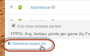
| 1. | Log into your FanDuel account and download the CSV relating to the contest you wish to enter.
To do this, choose the contest you wish to enter. After identifying the contest, click the “Enter” button. Once the contest loads, scroll to the bottom of the player salary list and click the link to “Download player list”. The file you download will have a unique name. Recall from our previous post on using CSV files that we will be better off to change this to a more generic name, like “FanDuel.csv”. We can then use that generic name going forward and instruct Excel to import “FanDuel.csv” each time it opens. By saving the file in the same spot and using the same name each time, Excel can seamlessly open and update the salary information with us not having to perform the CSV import each time. So, after you have renamed it, save your “FanDuel.csv” file somewhere you don’t mind it residing in the future. |
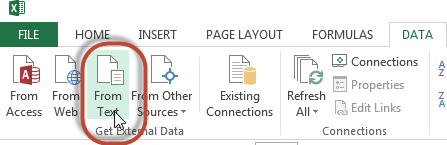
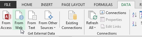
| 2. | Start a new Excel file or open the file you wish to add the FanDuel salary list to.
On Excel’s Data tab, click the “Get External Data From Text” button. Then browse to and select your “FanDuel.csv” file. Then hit “Import”. |
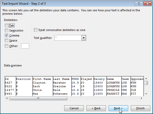
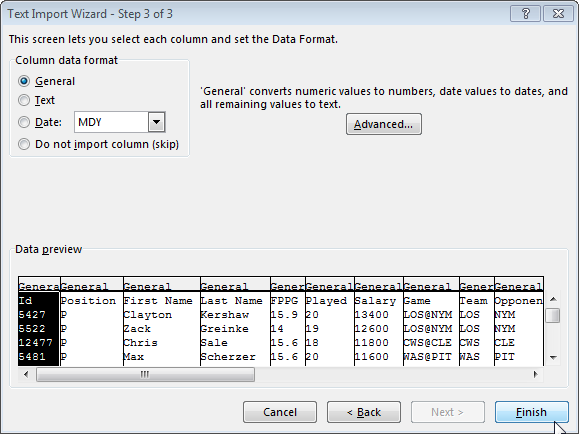
| 3. | At this point, Excel’s “Text Import Wizard” will open, asking you which type of file you’re importing. Choose the “Delimited” option and be sure to check the “My data has headers” box.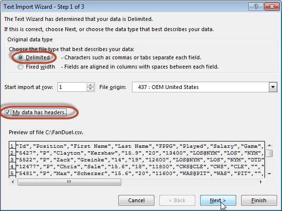
At step 2 of the import wizard, check the “Comma” delimiter box and uncheck any others. Click “Next”. No changes are necessary at step 3. Just click “Finish”. |
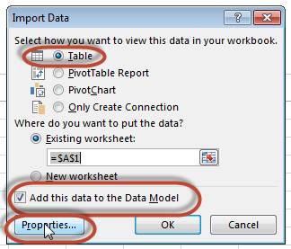
| 4. | This is where we diverge from the previous instructions. To format the imported data as an Excel table, check the “Add this data to the Data Model” box (other options on this screen will be grayed out until you check that option). Then ensure the “Table” radio button is selected under the “Select how you want to view this data in your workbook” area.
Click the “Properties…” button. |
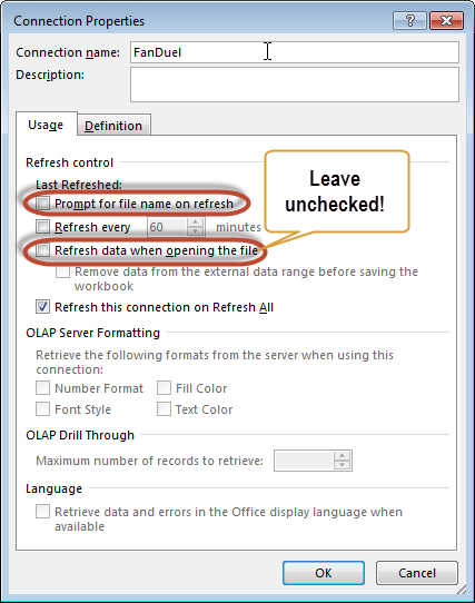
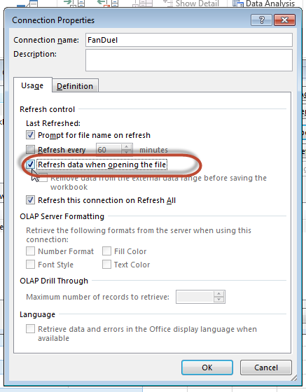
| 5. | In the past, I’ve suggested you check the “Refresh data when opening the file box” at this point. But don’t do that yet!
When I check that box at this point, my Excel file gets an error each time I open it. I get the sense the connection is still working, but the error bothers me. In researching the error, it seems others have experienced the same thing. The simple workaround to the error is to not check that box now, and just come back and check it later in the process. I would recommend unchecking the “Prompt for file name on refresh box”. Click “OK” to close the “Connection Properties” settings. Then click “OK” to close the “Import Data” settings. |
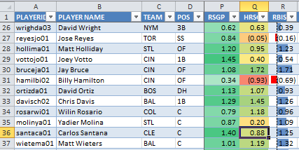
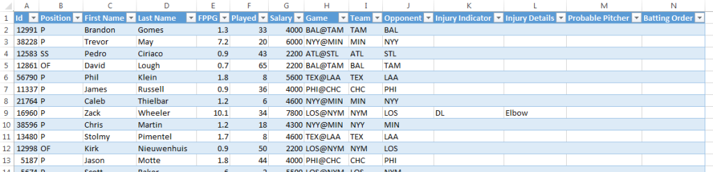
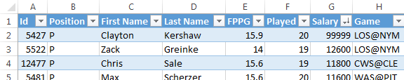
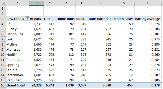
| 6. | Your import should be complete! You’ll know that Excel formatted your data as a table if it’s somehow shaded with alternating colors.
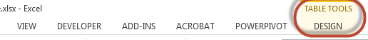
You can change the colors under the “Table Tools Design” tab that should appear on the Excel ribbon when you click within the table. |
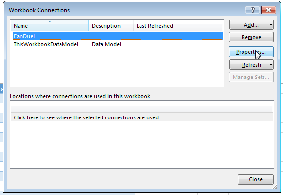
| 7. | After the import is done and you’re satisfied with the color, go to Excel’s “Data” tab and click on the “Connections” button.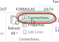
In the list of “Workbook Connections” that loads, choose your FanDuel connection and hit the “Properties…” button. Now check the “Refresh data when opening the file” option that we purposely held off on earlier. |
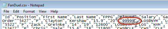
| 8. | To test the connection, close your Excel file. Then browse to and open the “FanDuel.csv” file.
Make an obvious edit to a player’s salary (for example, change Clayton Kerhsaw’s salary to “99999”), save your changes, and close the CSV file. Note, your CSV file may open in Excel. You can still edit a player’s salary. When you go to save the file, you’ll get a series of annoying messages about “Do you want to keep using the CSV format?”. Just be sure you’ve saved the file and say “Yes” to those questions. You’ll get prompted with the same set of questions when you close the CSV file. |
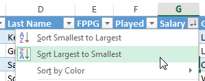
| 9. | Now open your Excel file and verify that the salary change you made flows through. You might first get a security warning from Excel that data connections have been disabled. Click the “Enable Content” button and watch the data below update.
My data files sometime import in a strange order. You may have to use the “Salary” drop down menu to sort by salary in descending order (to see Kershaw at the top).
|


Changing the Name of a Table
Now that you’ve created an Excel table, you an edit its name and other properties on the “Table Tools” tab. This tab is not always visible but should appear when you select a cell within the table.
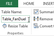
Once you’ve selected the “Table Tools” tab of the ribbon, you can change the name of the table under the “Properties” icon set all the way to the left of the tab. Remember, a great deal of the value from using structured references is the ability to use type ahead formula building and to have meaning in your formulas. So avoid names like “Table1” and go for things like “FanDuel_Salaries” or “Table_FanDuel”.
Using Type Ahead in Formulas
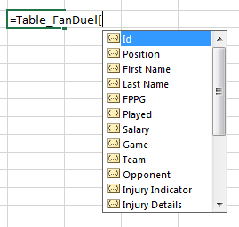
Once you’ve set up a table, the type ahead features immediately activate with no effort needed on your part. To see the type ahead in action, just start by typing the name of your table in a formula.
You can see in the image below that just typing “Ta” (for “Table_FanDuel”) pulls up the table. You can then use your mouse to double-click on one of the items in the list or use your arrow keys to select one and then hit the “Tab” key to select the highlighted item.
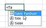
Once you have completed adding the table name, an open bracket (“[“) will then present you with a list of field names, all of which you can cycle through with the up and down arrrow keys and then hit Tab to select a column/field.
Wrapping Up
A little bit of a personal story here. I occasionally give Excel trainings at work to people that know their way around a spreadsheet pretty well. Most could even rattle off a VLOOKUP formula without much thought. I show them Excel tables and structured references and everyone’s eyes glaze over and they look like a bunch of deer in headlights.
I get it. The structured reference thing is new. If you already know how to do a VLOOKUP it’s hard to see the value in changing. Why take the time to do this?
Keep in mind that I try to design spreadsheets that will last for a long time and be reusable. At least for one season and possibly into future seasons. You could easily just get caught in a cycle of whipping up an inferior spreadsheet each time you want to create a lineup. But I would rather invest the time to build a long-term tool on a strong foundation. This way I can save time each night by having a prebuilt tool and because it’s built on a strong foundation I can continue to add new data, projections, and features over time.
And don’t you just love the pretty alternating row colors????
The SFBB way is all about doing things yourself, building things the right way, and continually improving and learning new things. So take the time to play around with structured references and learn the language.
Stay smart.


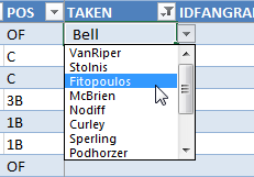
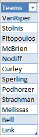 As I mentioned, this post assumes you have already added the named range and data validation drop down listing to select the team that has drafted a player.