Welcome to the sixth and final part of the “Create Your Own Fantasy Baseball Rankings” series. If you missed an earlier part, you can find it here. You can start at the beginning of the series or if you want to start here at Part 6, you can download the Excel file created during part 5 here.
Please note that this six part series has been adapted into a 10 part book that also shows you how to convert standings gain points into dollar values and how to calculate in-draft inflation.
A few notes about the series:
- It was originally written before the 2013 MLB season. The screenshots and player references you see might refer to things from that time frame, but the same approach will work today.
- If you register as SFBB Insider, you can receive all six parts in a free, tidy, and easy-to-use e-book
- Familiarity with Excel is recommended, but I do my best to explain all formulas and functions used
- Some of the formulas used in the series do not work in Excel for Mac computers. I apologize for this. I don’t understand why Excel isn’t built to operate the same on that platform.
In this sixth part of the series we will discuss the concept of replacement level players and calculating for position scarcity.
Replacement Level Players
Mike Trout is projected for 114 R, 26 HR, and 83 RBI. Those numbers are gaudy. But should he get “credit” for all those statistics if I can go out the day after the draft and pickup a player on the free agent list that is projected for 50 R, 15 HR, and 55 RBI?
This is the concept of replacement level. If player X is projected for 26 HR and there are several free agents that will hit 15 HR, the true value of player X is in his 11 additional HR (26 – 15).
So when calculating a player’s SGP, you should not perform the calculation on the “gross” or total number of HRs. Rather, you should calculate SGP with the amount of HR over a replacement level player (a free agent).
Determining Replacement Level
Assuming a 12-team league with 14 hitters (two C, 1B, 2B, SS, MI, 3B, CI, five OF, DH), 168 offensive players will be drafted (you can add more to adjust for bench players). So the 169th player is “replacement level”, right?
Arguably this is true. But let’s fine tune this a little more. In a 12-team league where each team must start two catchers, the 25th best catcher is the “replacement level catcher”.
If the league request one 2B, one SS, and one Middle Infielder, then 36 combined 2B and SS will be drafted. We can assume this will be comprised of 18 2B and 18 SS, and the 19th best of each position will be the “replacement level”.
Likewise, you might expect 18 1B, 18 3B, and 60 OFs to be drafted. But given that these positions typically produce better offensive statistics than 2B and SS, 1B and OF tend to be slotted into the UTIL/DH spots. This can push the 1B up to 24 selected players and the OF up to 66 selected players (with the 25th 1B being “replacement level” and the 67th OF being “replacement level”.
Let’s look at some projected statistics for Jason Heyward and Robinson Cano (please note the tables below don’t foot due to rounding) :
| Category | Heyward | Cano |
|---|---|---|
| R SGP | 3.82 | 3.58 |
| HR SGP | 2.60 | 2.40 |
| RBI SGP | 3.62 | 3.98 |
| SB SGP | 1.38 | 0.32 |
| AVG SGP | 0.12 | 0.96 |
| TTL SGP | 11.54 | 11.25 |
On the surface, the two are near equals, with Heyward holding a slight overall edge in SGP. But let’s now compare each to a replacement level player at their position. In my rankings spreadsheet, the 61st ranked OF is Ryan Ludwick.
| Category | Heyward | Ludwick | Heyward over Ludwick |
|---|---|---|---|
| R SGP | 3.82 | 2.32 | 1.50 |
| HR SGP | 2.60 | 1.92 | 0.68 |
| RBI SGP | 3.62 | 2.72 | 0.90 |
| SB SGP | 1.38 | 0.11 | 1.27 |
| AVG SGP | 0.12 | -0.14 | 0.26 |
| TTL SGP | 11.54 | 6.93 | 4.61 |
In my rankings spreadsheet, the 19th best 2B is Gordon Beckham.
| Category | Cano | Beckham | Cano over Beckham |
|---|---|---|---|
| R SGP | 3.58 | 2.20 | 1.38 |
| HR SGP | 2.40 | 1.25 | 1.15 |
| RBI SGP | 3.98 | 2.07 | 1.91 |
| SB SGP | 0.32 | 0.53 | -0.21 |
| AVG SGP | 0.96 | -0.35 | 1.31 |
| TTL SGP | 11.25 | 5.67 | 5.54 |
So despite a higher gross SGP (11.54 vs. 11.25), Heyward comes out as less valuable when we adjust for replacement level players. In fact, Cano moves to nearly one whole SGP of an advantage over Heyward (5.54 vs. 4.61). Continue reading “Create Your Own Fantasy Baseball Rankings: Part 6 – Accounting for Replacement Level and Position Scarcity”
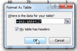


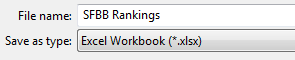
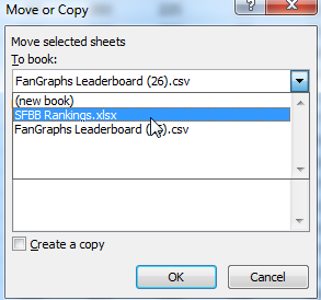
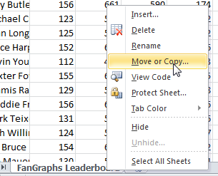 When prompted, choose your Rankings Excel file (saved in step 1 above) from the drop down menu. Then hit “OK”.