About a week ago I got an e-mail from a reader of the site asking me for help using “Power Query” to pull some Fangraphs data into Excel. Power Query is an add-in for Microsoft Excel that offers more advanced data importing options and ability to combine data from different resources.

I knew Power Query existed. But as I was reading the e-mail, my palms began to sweat and an overwhelming sense of guilt washed over me.
“I don’t know anything about Power Query!!!”
Coincidentally, my wife was out of town for the weekend and with the girls in bed early, I had a handful of hours on Saturday night to give myself a crash course in how to use Power Query (ah, the exciting and glamorous nightlife of a baseball nerd!).
And now I might be hooked.
Tables, Tables, Tables!!!
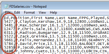
I recently wrote a post (about importing a CSV file into Excel) that included a list of benefit to using Excel tables.
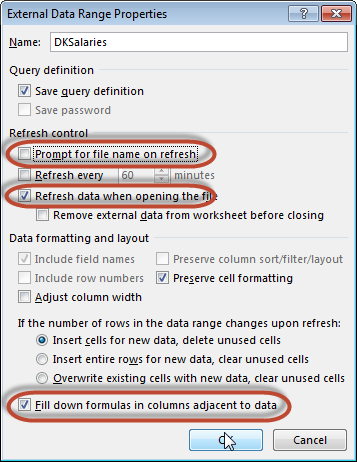
But I missed a really important one… If you import your data into Excel as a table, you create a connection to the data that is linked and can be updated automatically.
Let that sink in for a minute.
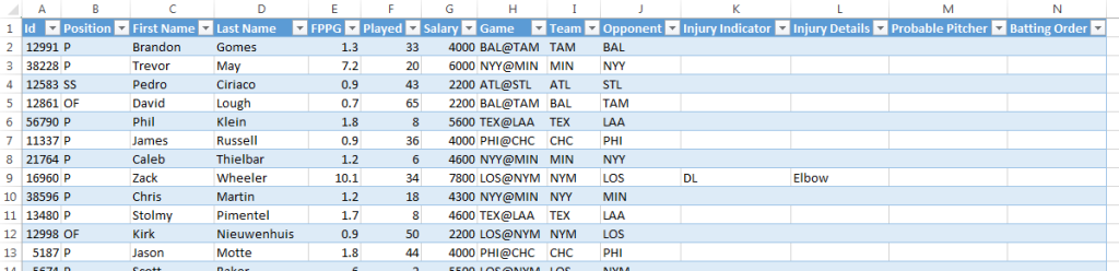
I’ve shown you how to make a lot of the Excel file’s that are isolated, dead, and not directly linked to any outside information.
I might have you download some data. Then copy and paste it into Excel. And then convert it into a table. But this is not ideal. The only way to update that information is to manually download it, open the file you downloaded, copy the data, paste it into your file, and cross your fingers that none of your formulas break when you paste over the top of everything.
If we can start importing data directly into Excel as tables, rather than copying and pasting data manually, we can maintain the link to the original data and then very easily update it in the future. And Power Query is capable of helping us do that. It gives more options to create live links to data sources and better options to manage those connections.
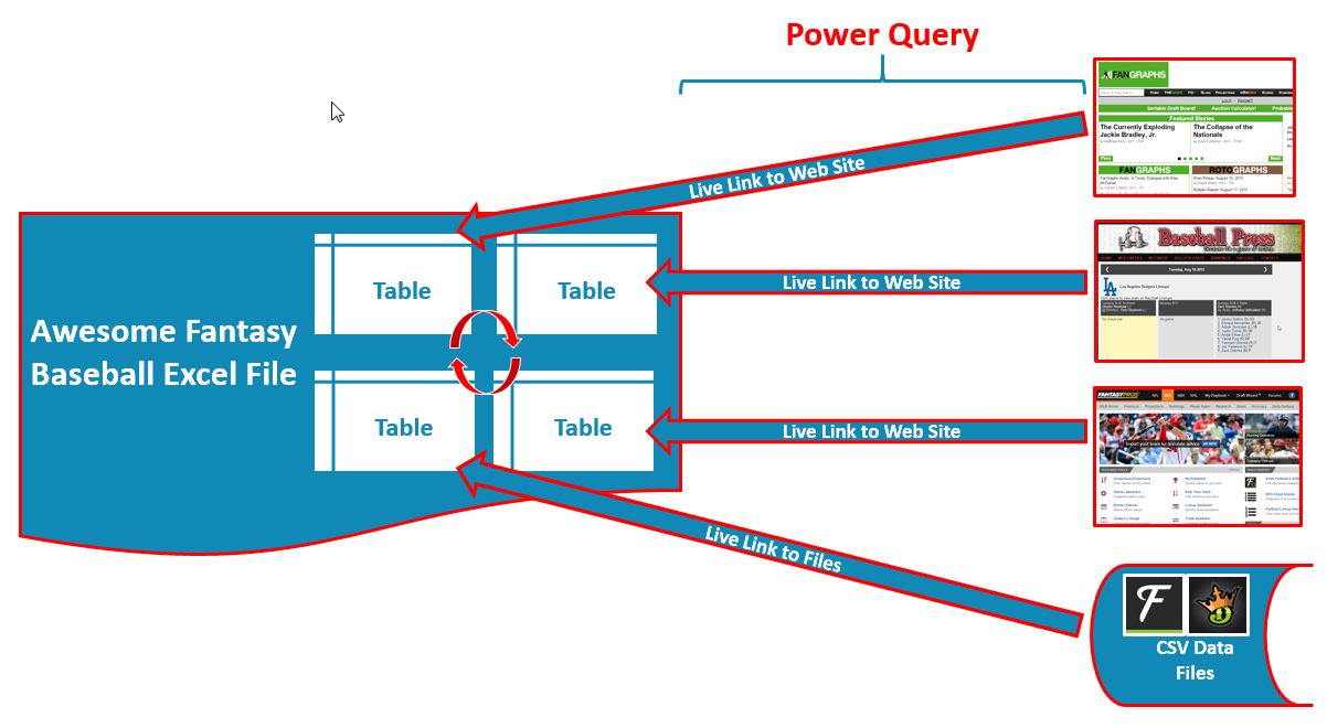
Imagine not having to rebuild a new rankings and dollar value file from scratch EVERY season. If you set the file up intelligently, you can use the same file to quickly get in-season values or to update the file for the next season in only a couple of minutes.
Power Query and the Power of Tables
In my limited use of Power Query so far, the thing that has me most excited is that it gives you the ability to import more data sources as tables. We have previously looked at how to use web queries to get information into Excel, but if you use a basic web query, the information does not come in as a table.
Granted, a web query does still leave a live link to the original data. But I want the best of both worlds. I want a live link to the original data AND to import it as a table!
There is a Catch
When using a standard web query (outside of Power Query), you do have the option to import the entire web page. This is messy and loaded with complications, but it’s helpful to have the option.
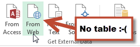
There is no such option in Power Query. You can only use Power Query to web query actual HTML tables from a web site. My educated guess is that to set something up as a table in Excel requires a neat and structured block of data, which querying an entire web page is not.
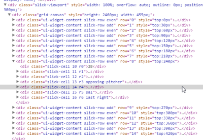
This is unfortunate, because some really great sites like Baseball Press don’t use tables to present their data. Instead, they use the division (< DIV >) HTML tag.
Downloading Power Query
Despite Power Query not being the silver bullet we need to resolve all our data needs, it’s definitely a tool worth having in the arsenal. And it’s free!
You can download the add in from this page. There are some restrictions you should know about. The program requires at least Windows 7 (sorry again Mac users… you should really look into partitioning your Mac to run Windows).
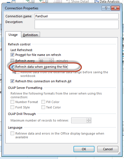
You also need to be running Excel 2013 (any version) or Excel 2010 “Professional Plus”. After you’ve downloaded the installation, close out of Excel and proceed through the installation. The new toolbar on the ribbon should appear the next time you open Excel. If you’re not seeing a “Power Query” tab, you may need to activate the add-in. Check out the instructions here on how to turn on the add-in (look for the section labelled “My Power Query Tab Disappeared”). ![]()
Making Your First Web Query With Power Query
If you’ve read any of my previous pieces on web queries, this really isn’t that much different. The improvement is with the data being in a table and some additional capabilities to fine tune the data that is imported. But let’s take a closer look at how the basic functionality changes.
| Step | Description |
|---|---|
| 1. | The first task is to identify a web page you want to query AND to determine that it does contain HTML tables. My excitement over Power Query is tempered some by that fact that it is difficult to locate useful resources that put their data into tables. Many valuable sites and specific pages don’t!
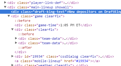
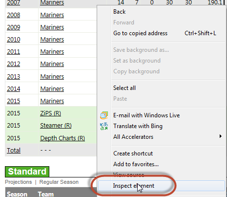
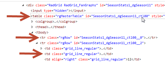
Remember, to determine if data is in a table, right click somewhere on the web data you would like to capture and choose the menu option to “Inspect Element”. This will load the HTML “code” used to create the web page. If you see references to A few examples of potentially helpful tables that I’ve found:
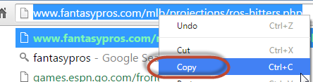
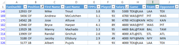
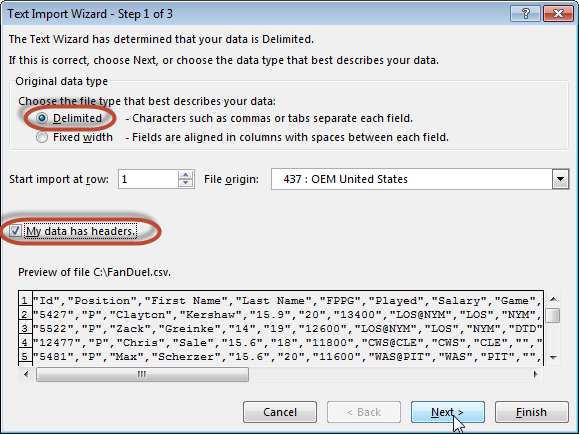
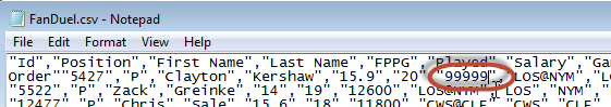
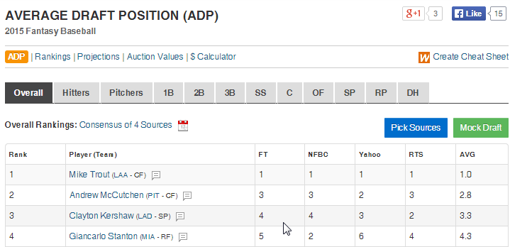
After you have located a table to import, copy the web page address. For my example, I’ll use the Fantasy Pros rest of season projections (link is http://www.fantasypros.com/mlb/projections/ros-hitters.php). I realize this is not useful for DFS, but I just want to demonstrate the basics of Power Query now. |
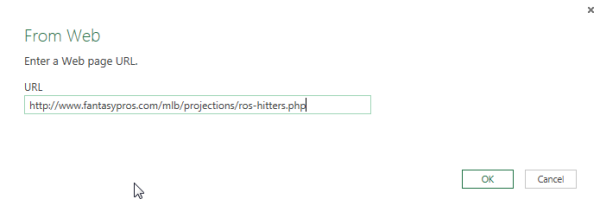
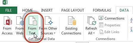
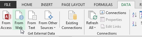
| 2. | Open a blank Excel file. Click the newly added “Power Query” tab. Then click the “From Web” icon on the left of the ribbon.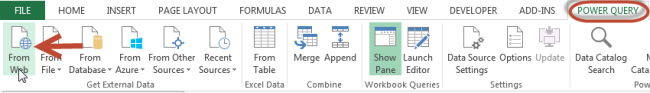
Then paste the copied URL into the dialog box and click “OK”. |
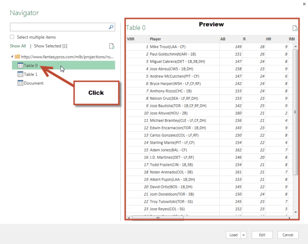
| 3. | The “Navigator” dialog will appear. It may take a minute or two to load as Excel processes each of the tables on the page.
Once the loading process completes, you will see a list of all the tables available for import. Click your mouse to locate the data you want. If you wish to import more than one table, check the “Select multiple items” box. As you click on the various tables, watch the preview pane on the right in order to locate the exact table you want. |
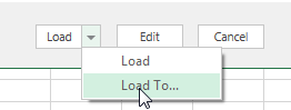
| 4. | Stop! This step is informational only. Don’t do anything!
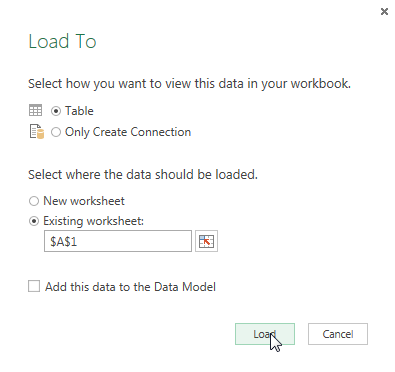
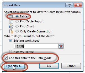
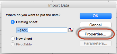
At this point, you could click the “Load” or “Load To…” button. The “Load” button will import the data exactly as you see it into a newly created worksheet tab. The “Load To…” option gives you a few more control over how the data loads. In the ensuing menu you have the option to import the table (recommended) or only add the connection to your file (not sure why you would want to do this unless you were unsure of where to place the table now). You can also choose to create a new worksheet or to place the table in an existing spot. Working with data models is something I may explore in the future. If you want to look ahead, you can start here Loading from here bypasses some of the real value that Power Query offers. These features are available when you click the “Edit” button. |
| 5. | Start! You can start following along again.
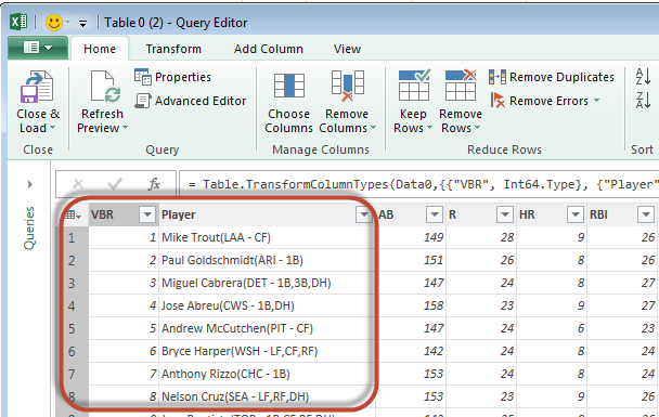
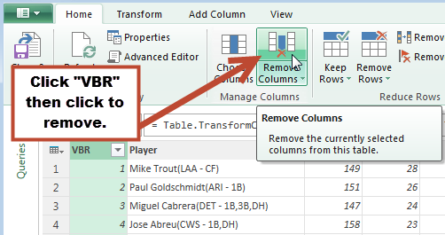
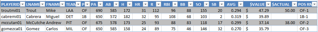
Click the “Edit” button and the “Query Editor” will load. In this screen we not only see the preview of the data that will be imported, we can also clean things up. For example, the first column is labelled “VBR”. This looks like some kind of a ranking, but I don’t want to import this. Additionally, the second column has a lot of information in it. Instead of seeing “Mike Trout(LAA – CF)” all in one column, I want to try breaking that into separate columns. Rather than bring it in and have it clog up my screen, we can tell Power Query not to import this column. To do this, click on the “VBR” column to select it. Then click the “Remove Columns” button. |
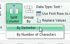
| 6. | Now let’s move on to splitting apart the player name, team, and position.
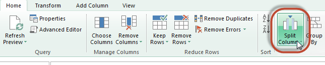
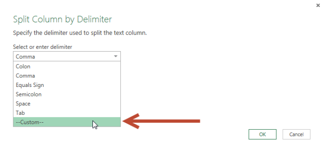
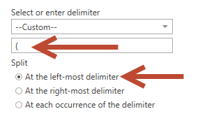
Click once on the “Player” column. Then click the “Split Columns” button. And then click the “By Delimiter” option. A delimiter is a unique character that represents a change in the field or information. Looking at the data we have, the opening parenthesis is a delimiter between player name and team. There is no option to choose that from the drop down menu, so instead select the “–Custom–” option. Then type in the open parenthesis, “(“, and select the option for “At the left-most delimiter”. You should now see that the columns automatically get split! |
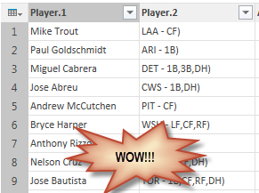
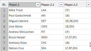
| 7. | Let’s keep going and try to separate out each player’s position. Click the new “Player.2” column and then click the “Split Columns>By Delimiter” menu button again. This time use the settings in the image below to split the column at the hyphen.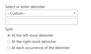
Power Query is really looking useful. |
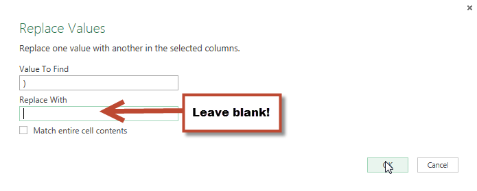
| 8. | The last thing bothering me is the closing parenthesis after each player’s position. To get rid of this, click to select the “Player.2.2” column and then click the “Replace Values” icon.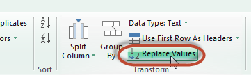
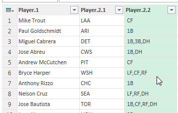
Once the “Replace Values” dialog loads, enter the closing parenthesis in the “Value To Find” field AND LEAVE THE “REPLACE WITH” FIELD BLANK! Then click “OK”. Check this out… |
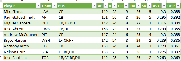
| 10. | Now that the data is cleaned up, click the “Close & Load To…” button on the “Home” tab of the ribbon.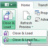
This will load the same “Load To” box discussed earlier. Adjust the settings as you see fit and click the “Load” button when you’re done. The data loads exactly as you cleaned it up! |
 .
. 
This Is Not the Best Example
Because I’m in the middle of a series of DFS-related blog posts, I wish I had a more concrete example that specifically tied in DFS information. But I did want to demonstrate the power of cleaning and tweaking data with Power Query. Hopefully you can recognize there is a great deal of value in knowing these tools exist so you can use them to solve issues as you build your own DFS spreadsheet with the information you like using.
I’ve included a couple more links below that may help you down the Power Query path.
As always… stay smart.
Are You Using Power Query? Other Add-Ins?
Is anyone using Power Query already? What kinds of things are you using it for? What sites are you loading the data from?
I’d love to hear it if you are. Please e-mail me or leave a comment below.
Other Resources
I’ve only given a brief overview of the full capabilities. If you’re intrigued and looking for more examples, check out these additional resources below.
| Name | Description |
|---|---|
| Download Page | Free download page. Power Query is free, but it does require you to have Excel 2013 or Excel 2010 “Professional Plus” (I don’t know exactly what that means). It also requires you be using at least Windows 7.
If you’ve been on the fence about upgrading to the newest version of Excel, I list out a few of the purchasing options here. |
| Interactive Online Tutorial | If you choose only one of these items to click on. Choose this one. The demo is only a few minutes long, but it does a great job of demonstrating how you can really fine tune and clean up the data you import through Power Query. |
| Interesting Examples that Might Apply to Baseball Data | This is a fairly lengthy post, but look specifically for the sections labelled “Append (Combine) Tables with Power Query”, (I could see this being a way to import a player’s last three seasons of data, or to import multiple projection systems) and “Merge Tables – A VLOOKUP Alternative” (a way to combine DFS salaries with info from other sites). |
| Introduction to Power Query | This is simply a written explanation of Power Query and its features and benefits. More detailed than I’ve explained above. |
| Advanced Example, Dynamic and Multi-Layered Queries | I started this post off by referring to a question I received from a reader of the site. He wanted to provide Excel with a list of player IDs and then have it systematically go out to the player pages for each of those IDs and pull back data.
I wasn’t sure this was possible in Excel, but turns out that it is! This resource demonstrates how to make advanced edits to your query to make it dynamic (to ask for a player ID) and to make it multi-layered. Said another way, you can have one query go and fetch a list of player IDs and you can have a subsequent query run off each of those IDs. “Hey Excel, go get this list of players. Then go through each player on that list and go get me the standard data from their Fangraphs page.” It’s slow… But it works. |


 Copy this information and go to your “Hitter Ranks” tab and paste it into the first cell below the header in column A there.
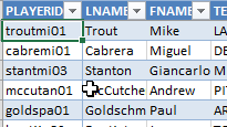

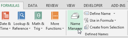
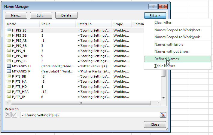
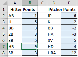 To refresh your memory and to see the complete list of named cells, access the “Formulas” tab of the Ribbon and then click the “Name Manager” button.