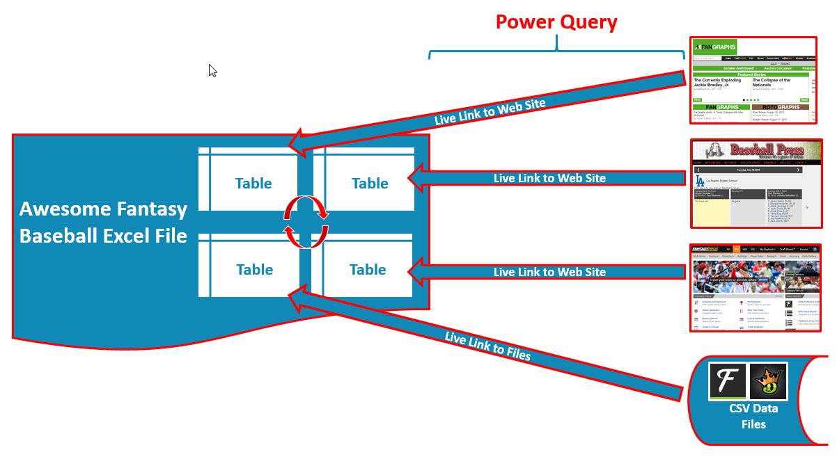
In this post I’m going to address two common questions I get about creating daily fantasy baseball spreadsheets:
- Where and how can I download today’s AND tomorrow’s projected starting pitchers?
- Why I don’t see the yellow arrow when trying to web query a site in Excel?
And in addressing those two questions, we’ll also take a look at a powerful tactic of using Google Sheets and Excel together to get baseball data off the web. We’ll be focusing closely on obtaining a list of projected starters, but the concepts behind using Google Sheets and tying that back into Excel is one that can be applied in many other areas (like creating spreadsheets for your season long leagues).
Where Can I Find a Reliable and User-Friendly List of Probable Starting Pitchers?
We all know DFS is exploding and there are countless sites out there providing lineup information, alerts, weather data, and more. But unless I’m looking in the wrong spot, most of that information is intended for that day’s games. And as a father of two with a day job, I can’t practically create a lineup the day of a contest. I need to prepare a day in advance for the next day’s games.
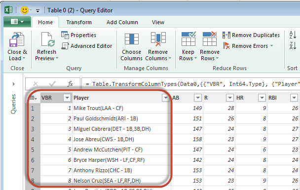
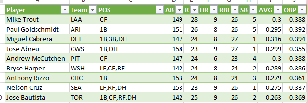
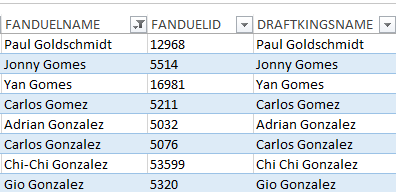
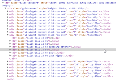
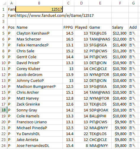
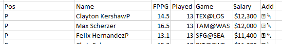
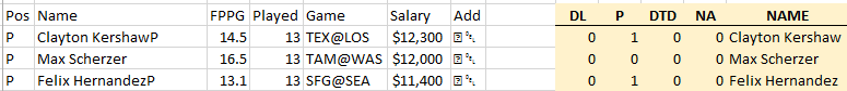
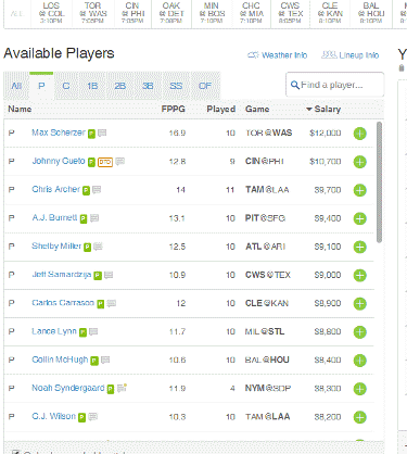
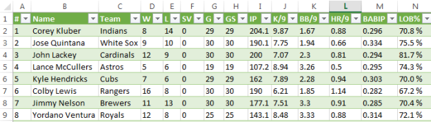
The other challenge in finding this information is that it will be a lot easier to deal with in Excel if we can find the data in a table format (see image to the right, I won’t bore everyone with technical details, but just because data looks to be in columns and rows on a site, doesn’t mean it’s in the format Excel can handle easily).
I have struggled and struggled to find a good resource for tomorrow’s projected pitchers. AND IT HAS BEEN RIGHT IN FRONT OF MY FACE ALL SEASON! Take a look at the Fangraphs home page:
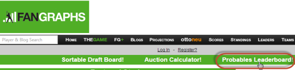
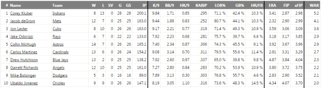
If you visit the “Probables Leaderboard” (here’s an example link), it looks perfect. A table of all the projected starters, and even some friendly advanced metrics we could use in evaluating each player.
Now take a look at the URL for the page:
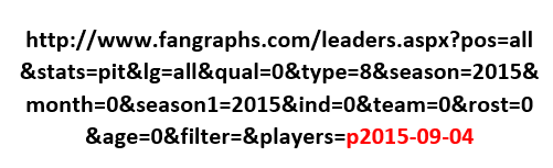
I started to write this post on September 4th. And when I clicked the “Probables Leaderboard” link, it took me to the “p2015-09-04” web address. You can see that last part simply reflects the current date.
Anytime you see a URL like that, with all the different arguments and parameters (like “pos”, “stats”, “lg”, “season”, etc.), you should get excited. It likely means you can manually type in values for those parameters and create your own “query” of the site. Here’s an example I wrote awhile back using Brooks Baseball to illustrate these concepts.
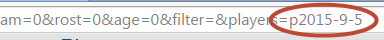
So instead of just using the “p2015-09-04” address, I tried “p2015-9-5”. This was to test two different things. First, to see if I could get tomorrow’s probables in the same table format. Second, to see if the zeros before the month and day numbers were important… And it worked!
So not only do we have a reliable list of probable starters, we can also get the projected starters for days in advance!
We Need a Dynamic Web Query
While it’s great that we now know where to get tomorrow’s probable starters, the fact that the URL changes each day is a challenge. We’ll need to create a dynamic web query that can determine tomorrow’s date and download the data from the appropriate web address.
With this in mind, I brushed up my memory on how to create a dynamic web query (look for the section titled “Step-by-Step Instructions, Dynamic and Updating Web Query”) and started the process of building it in Excel.
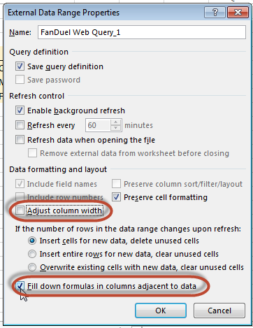
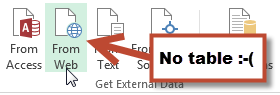
Why Don’t I See the Yellow Arrow in My Excel Web Query Window?
Everything was going so well until I hit a common stumbling block that occurs when web querying in Excel. No yellow arrow displays on the table of data I want to capture in my web query. ![]()
Why does this happen? One definite cause is if the information isn’t really in HTML table format (remember that image above?). But the Fangraphs table is in fact a table. I checked. I don’t have a great explanation as to why you don’t always see the yellow arrow, but I imagine it has something to do with how the table is coded or just Excel’s ability to properly process it.
But if you do in fact see that the data is stored in an HTML table, Google Sheets offers a very simple method of doing a web query. One that works even when the yellow arrow box is missing!
Why Don’t You Use Power Query?
That’s a really good question. I just spent thousands of words spouting the virtues of Power Query, and in my next post I turn my back on it?
I would like to. But the dynamic web address tripped me up. I spent three days trying to figure out how to get it to work and was unsuccessful.
I ultimately realized that I knew a much easier way to do this with Google Sheets, and this is something I’ve been meaning to demonstrate for a long time. So rather than continue to waste time trying to get Power Query to do the job, why not go with something I already know?
The ultimate irony of the situation is that Power Query didn’t have a problem importing the probables! If I could only have gotten a dynamic query to work…
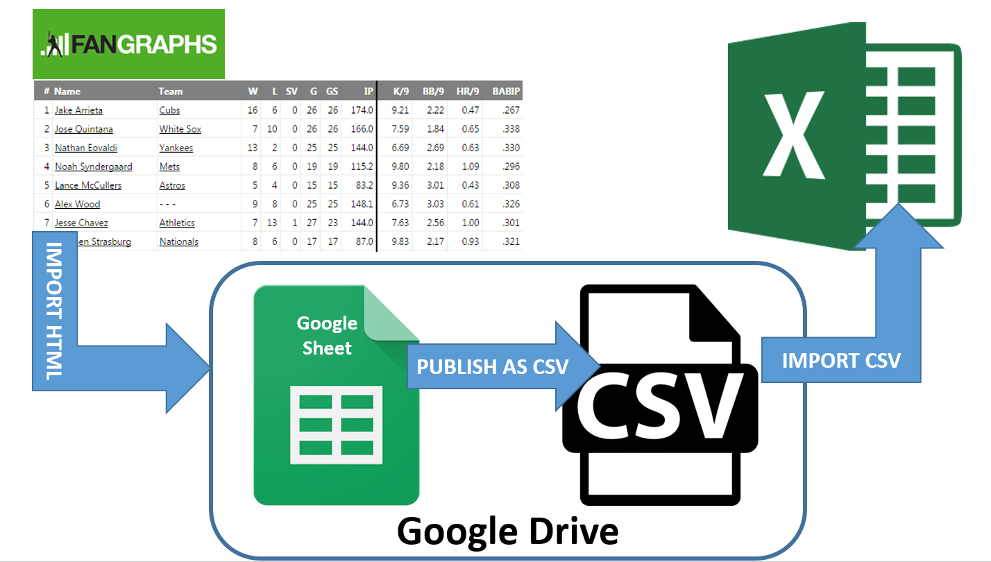
Enter Google Sheets
If you’re not familiar with Google Sheets, it is a very strong spreadsheet alternative to Microsoft Excel. And it’s free.
So why don’t I write more about using Sheets? Quite frankly, Excel is the better product. It is much more powerful and responsive, largely because it’s an application that runs on my own computer. Google Sheets is web-based and suffers from performance limitations and access issues because of it (if you have a slow internet connection or a lot of calculations in your spreadsheets, you’ll drive yourself crazy using Google Sheets).
With that said, there are some really interesting benefits to Google Sheets. Being free is hard to beat. It’s very easy to share a workbook and work on the spreadsheet at the same time as others. And as I mentioned, importing HTML table data is a snap!
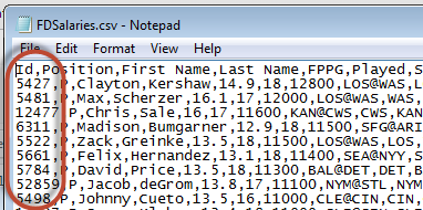
Another really neat feature is that you can publish (or share) the results of a spreadsheet online in CSV format.
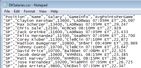
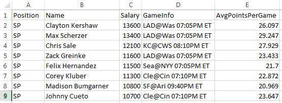
And a file in CSV format is easily importable into Excel!
So we can create a Google Sheet to web query troublesome table data. Publish that data as a CSV. And then use Excel (and even Power Query) to import the data into our master spreadsheet.
Let’s get started!
Prerequisites
To use Google Sheets, you need to have a Google account (if you use Gmail, Google Drive, or any other Google service beyond searching the web, you already have one). If you don’t have a Google account you can create one from the Google Sheets sign up page here.
Google Sheets Functions Used in This Post
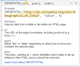
IMPORTHMTL
In Excel, we set up a special connection to pull information from a website. Things are much simpler in Google Sheets. You enter a very simple formula and the data gets pulled into the document.
The specific function we’ll use is “IMPORTHTML”. The function has three inputs:
- URL – Enter the web address of the page to be queried in quotation marks. In our example, it will be the address of the Fangraphs Probables page.
- Query Type – This is the data type you wish to pull from the web page. You can enter either “table” or “list”. Similar to what we look for when doing an Excel web query, we most likely will be using the “table” option.
- Index – This is the instance number of the table (or list) on the web page. Google’s documentation says the index begins at 1, meaning if you want to query the first table on a page you would simply type a 1. If you want the fourth table on a page, you’d enter a 4. But for some reason using a 0 is what works for the Fangraphs page we’ll be using.
MONTH, DAY, and YEAR
These are three separate functions. Each is looking for one input, a date.
The MONTH function will return the numeric representation of the month in the date. DAY returns the numbers from the date string corresponding to the days. And YEAR returns the numbers of the year in the date.
Going back to our example date string from earlier, a formula of =MONTH("09/04/2015") will return “9”.
TODAY
The TODAY function requires no inputs. And when used it simply returns today’s date.
For example, if you enter the formula =TODAY() and look at your spreadsheet on September 5th, 2015, your spreadsheet will display “9/5/2015”.
The formula updates when your spreadsheet recalculates. So if you opened the spreadsheet the next day, the formula would display “9/6/2015”.
You can perform addition with the TODAY function. So if you wanted to display tomorrow’s date, the formula would be =TODAY()+1. Or a week from now would be =TODAY()+7. Knowing that we can add one to the TODAY function will be important to finding tomorrow’s probable starters.
CONCATENATING or BUILDING TEXT STRINGS
By now you probably realize that we’re going to take the beginning of that long Fangraphs URL and then attach the date, as calculated by the TODAY function, to that. Every day these formulas will update and automatically create the new URL to determine tomorrow’s pitchers.
To attach two strings of text together in Google Sheets (or in Excel), you can use the ampersand (“&”). For example, we could put tomorrow’s date in cell A1 of a spreadsheet and then use this formula to build the Fangraphs web address:
="http://www.fangraphs.com/leaders.aspx?pos=all&stats=pit&lg=all&qual=0&
type=8&season=2015&month=0&season1=2015&ind=0&team=0&rost=0&age=0&filter=&players=p"&A1
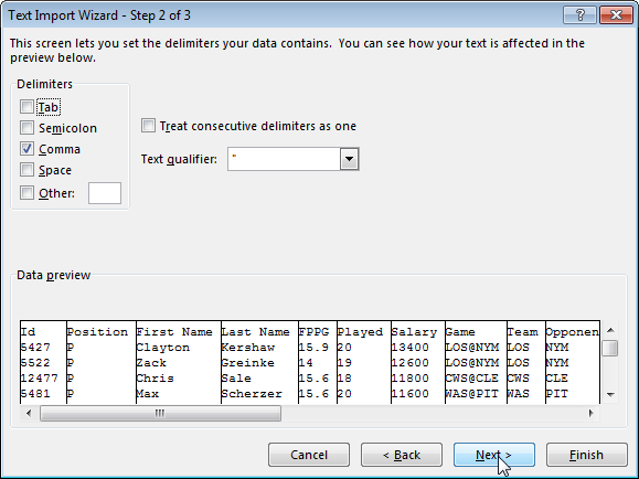
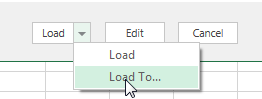
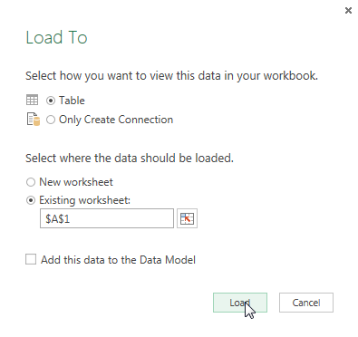
Step-by-Step Instructions – Create a Google Sheet and Use the IMPORTHTML Function
| Step | Description |
|---|---|
| 1. | Go to the Google Sheets home page and click the button to start a new blank spreadsheet.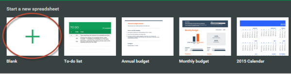 Click on the “Untitled spreadsheet” title and give the file a better name. Maybe something like “Tomorrow’s Probables”. 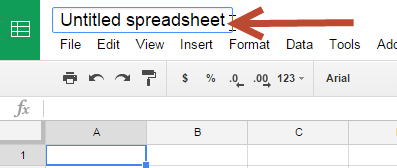
|
| 2. | Next, we’ll use the date formulas previously discussed to build the date string to attach to the Fangraphs probable starters URL. Enter the following formula in cell A1:
This should result in just the year of today’s date. As I write this post in September of 2015, the formula returns “2015”. Now we’ll continue to build on this formula. Add the following to the existing formula in cell A1:
Hit ENTER to accept your changes. See how the ampersand is used to add the hyphen and then another ampersand is used to add the month? As I write this post, that last formula results in “2015-9”. We’ll continue to use the ampersand to add new pieces of text to this string. Now add the following to the end of the formula:
This last piece puts in one more hyphen and then the current day of the month. In my example file it’s showing “2015-9-5”, which is the exact format we need for the Fangraphs page. But remember, we want to show tomorrow’s date. Not today’s. So make these last final adjustments:
The reason we have to add one to all three pieces of the date is to account for when you reach the last day of a month. If you don’t add one to the month component, your day would reset to “1” but your month would still be lagging one behind (e.g. If it’s August 31st and I don’t add one to all of the today formulas, my formula would results as “2015-8-1”, not “2015-9-1”). |
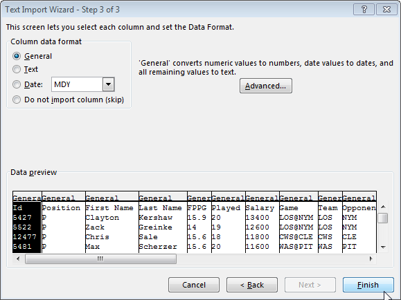
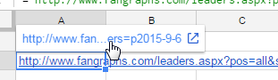
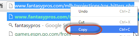
| 3. | We’ve completed the last date piece of the Fangraphs web address, so let’s create the full address to the page so that it will update dynamically. Visit the Fangraphs probables page (here’s a link you can use that will lead to an old date). Use your mouse to select all but the end of the URL that contains the date (get the “p” though!).  Copy that URL. Then return to your Google Sheet. In cell A2 type an equal sign then a quotation mark:
Then paste the Fangraphs URL and close it with another quotation mark:
Now use an ampersand to append in cell A1 (the missing date component to the end of this formula):
Hit ENTER to complete the formula and you should see a fully usable hyperlink that will take you to tomorrow’s probable starters. |
| 4. | There are just two more inputs needed for the IMPORTHTML function. Type TABLE into cell A3 and a zero into cell A4.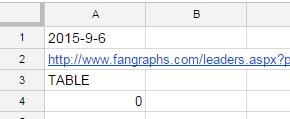 Now click the downward pointing arrow on the sheet name at the bottom of the screen and then choose the menu option to “Rename…”. 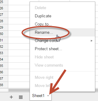 Give this tab or the spreadsheet a meaningful name, like “IMPORTHTML Inputs”. 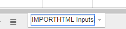
|
| 5. | Now click the “+” sign, to the left of this newly renamed tab, in order to start a new sheet.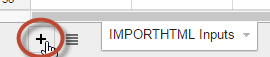 Click the downward pointing triangle on this new sheet and rename it to something meaningful, like “Probable Starters”.  |
| 6. | Click your mouse into cell A1 and enter the following formula:
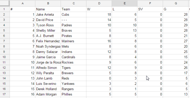
If you named your first tab exactly the same as I did, you can copy and paste the formula above into cell A1. Or instead of typing out the formula, you can click to your “IMPORTHTML Inputs” tab and select the applicable cells. Hit enter to accept the formula. After several seconds (depending on the speed of your internet connection), you should see the probable pitchers load! You can see that it’s very easy to pull data from the web into Google Sheets. Much easier and with fewer steps than in Excel. |
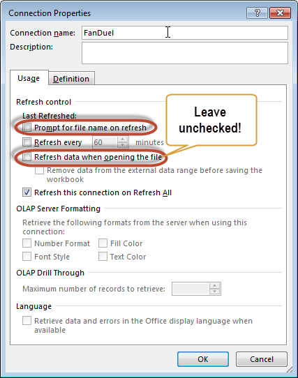
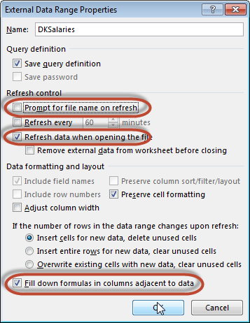
| 7. | Before we go on, think for a moment about how an Excel spreadsheet runs its calculations. Similar to Google Sheets, Excel has a TODAY calculation. But if the Excel file containing the TODAY formula was closed for an entire week, we wouldn’t expect that the TODAY formula was updating each day in that closed spreadsheet.
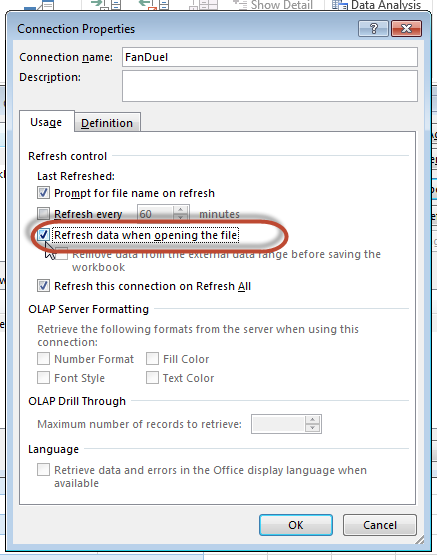
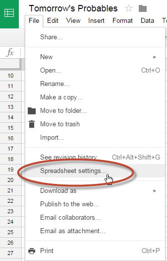
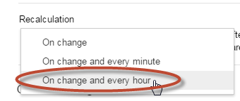
We face a similar problem with this Google Sheet. We don’t want to have to open this list of probable starters each day just so it can update the list. It would be great if there were a property we could turn on so that the spreadsheet would refresh itself every so often… And fortunately Google offers this feature! Within the Google spreadsheet, go to the “File>Spreadsheet Settings…” menu. In the ensuing menu, adjust the “Recalculation” setting to the “On change and every hour” setting. This means the spreadsheet will reevaluate the TODAY formula each hour and update the list of probable starters accordingly. Click the “Save settings” button to accept this change. |
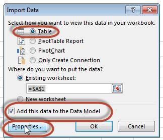
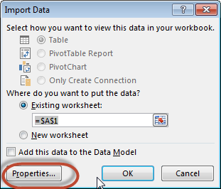
| 8. | The last task we need to complete in the Google Sheet file is to publish the list of starters as an online CSV file.
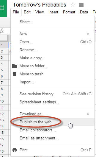
To start this process, click on the “File>Publish to the web…” menu. |
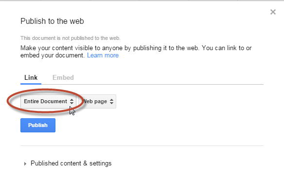
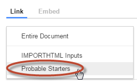
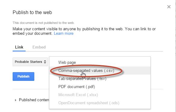
| 9. | After you click the publish button, the menu will change to display a link to the published CSV file. Copy this link for now. We’ll need it in the next section. In fact, you may want to copy and paste it into a Word file or some other place for easy access. We will use it again a couple of times.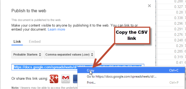 You can always return to review or change these settings under the “Publish to the web…” menu. Just click the “Stop publishing” button, reconfigure the settings to your liking, then republish the document. 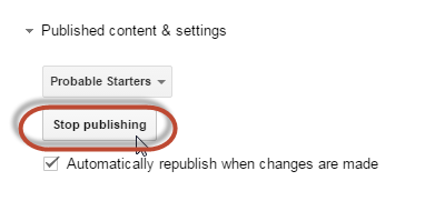 |

Google Sheets Wrap Up
Now you see how much more simple the “web query” is in Google Sheets. Especially the creation of a dynamic query that can grab the results of a different page each day with no need for us to update or even open the file! When a new day rolls around, the probable starters list will automatically update in the Google Sheet and in the published CSV file.
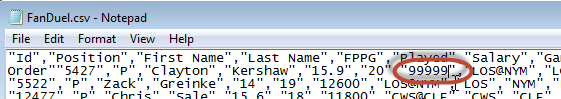
The ease of importing data is a huge benefit of Google Sheets, but on the whole I don’t find it to be up to par with Excel. So now let’s take a look at how to get this CSV file into our daily fantasy baseball spreadsheets.

 .
.