I’ve recently made some notable edits to the Player ID Map that should be helpful to many.
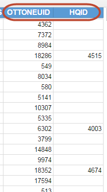
Added a field for “OTTONEUID”
Added a field for “HQID” (for Baseball HQ player IDs)
Updated “POS” column to reflect games played during the 2015 season. I determine which positions a player qualifies at using a 20 game minimum and then assign the player to ONLY his most valuable position. I assume position value goes C, SS, 2B, 3B, OF, and then 1B.
Added several new players
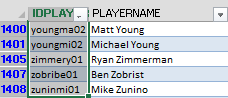
The Ottoneu ID column is almost completely full of IDs, there were very few players I had on my list that are not in the Ottoneu universe. In fact, I think it’s just the foreign players coming to MLB for the first time this season (Maeda, Park, etc.). The Fangraphs IDs for those players recently became available and they ARE now included in the map.
The Baseball HQ ID column is not nearly as populated. It only includes about 450 or so players that I think are included on one of HQ’s current year rankings files.
I’ve also added players like Zach Davies, A.J. Reed, Max Kepler, Tim Anderson, Orlando Arcia, Trevor Story, and Adam Conley.
Player Name
Fangraphs ID
Kenta Maeda
18498
Byung-ho Park
18717
Hyun-soo Kim
18718
Orlando Arcia
sa596917
Tim Anderson
sa737508
A.J. Reed
sa599279
Max Kepler
12144
Zach Davies
13183
Trevor Story
sa597765
Adam Conley
14457
As usual, if I’m missing a player or if you find an error on the log, please e-mail me or send a Tweet to @smartfantasybb with the information. I do try to keep the log current with “fantasy relevant” players. But that definition gets real cloudy when I start to consider DFS.
I’ll try to add these new ID systems to the Projection Aggregator soon, but I think HQ reports typically include “MLBAM ID”, so you can always use that instead.
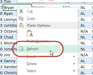
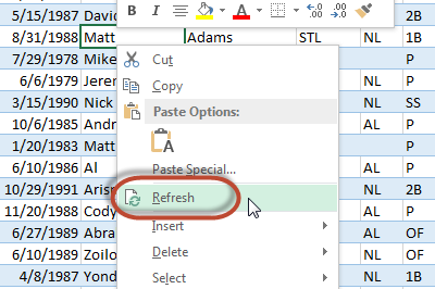
If you have Excel 2013 and you’ve downloaded the “new” version of the Player ID Map, you can right click anywhere in that tab of the spreadsheet and choose to “Refresh” the connection. Excel will seamless download the new updates to your file.
Let me come clean. I screwed up. And it likely will cause you to see errors in your spreadsheets. That’s the whole reason for this post.
Having trouble with VLOOKUP error messages? This post should help.
What Happened?
While this post is going to address a very important topic (resolving VLOOKUP errors), there wasn’t much of a need for this until I came up with a new format for the Player ID Map. The intent was to make the Player ID Map easily updatable. I hate having to lookup the IDs, birth dates, and handedness of all the new players.
And it’s always bothered me that there was no easy way for you to get updated Player ID information.
Let’s be honest. It’s a pain in the ass. Especially this time of year when players are switching teams every day and minor league players we haven’t had to deal with in the past are now projected to reach the big leagues this season. It’s tedious to keep teams up-to-date and to add these new players.
I needed to find a way to improve this process and to make everyone’s lives a little easier.
The Solution
The solution was to make the Player ID Map available in an online CSV file. One you connect that online file to your Excel spreadsheet, you simply have to right-click on the Player ID Map and hit “Refresh”. You will instantly get any update I’ve made.
Sounds amazing, right?
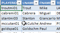
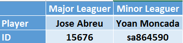
Major leaguers have a purely numeric ID while minor leaguers have text in their ID.
The Problem
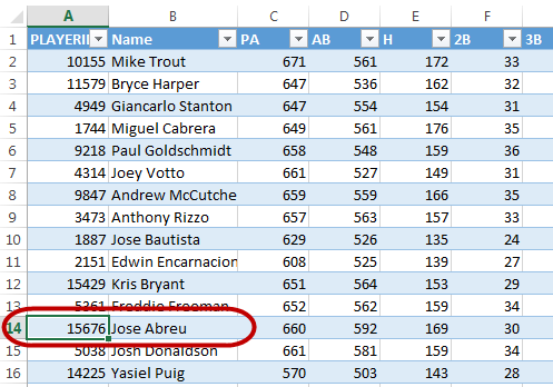
The fly in the ointment happens to be the way Fangraphs structures their player IDs. Major leaguers, like Jose Abreu, have a purely numeric ID. Whereas minor leaguers that have not reach the big leagues, like Yoan Moncada, have the text “sa” in front of a string of numbers.
The unintended consequence of importing the Player ID Map file is that because some IDs contain text, Excel will treat the ENTIRE imported column as text.
The problem is that reports you download from Fangraphs and then open in Excel treat the player ID column as numeric values.
Warning… It’s About to Get Technical
If you’re fine with the old Player ID Map and the fact that it doesn’t get updated very often, you don’t have to use the new one. The old one can be downloaded here and will still be updated periodically. You can stop reading this post and save yourself some sanity.
But if a little complication doesn’t scare you off and you see the value in being able to refresh the Player ID Map and get regular updates… Keep reading.
Text and Numbers Are Treated Differently
Excel and most other computer applications treat text and numbers differently. And this is a common problem with VLOOKUPS. So the number “15676” is not the same as a text string of “15676”. So in our VLOOKUPS, we need to make sure we are comparing numbers to numbers and text to text.
Consider the Error Message
The first step in resolving a VLOOKUP problem is to understand the error message you’re seeing.
The “#N/A” error is the most common VLOOKUP error. And it essentially means that a match was not found during the lookup.
There are two main reasons a match would not be found:
The item (player ID) doesn’t exist where you told Excel to look for it
Or you told Excel to look for the wrong data type (look for a text value in a list of numbers, or vice versa)
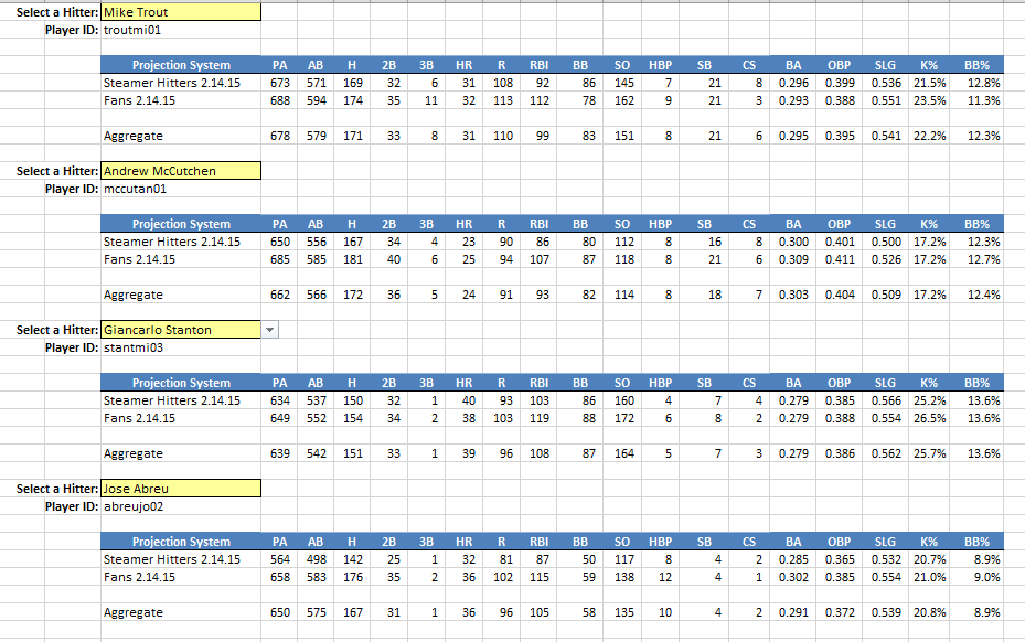
Abreu’s ID is the there. It’s in the first column. Why isn’t the VLOOKUP finding this???
You can easily test the first error by manually performing the search yourself. Let’s walk through a hypothetical example with Jose Abreu. He’s a well known player. He’ll surely be in the Steamer projections I’ve downloaded.
I see from the data that Abreu’s Fangraphs ID is 15676. If I trace that through into the Steamer Hitter projections, I am able to locate Abreu. So why isn’t the VLOOKUP finding the same match?
I’m a little biased, but I think the Player ID Map is an invaluable tool.
But if I’m being honest… it has a really big weakness. When I make changes to it, there’s not a great way for me to get that updated information to you.
The advantage of doing this is that you can link to this Google Sheet in your own spreadsheets. And if you download the Excel version, it will already have a pre-established link to the Google Sheet version.
How to Update the Player ID Map
Once you’ve downloaded the new version, you can simply right-click anywhere in the player listing and choose the option to “Refresh” the connection. Any changes will automatically pull into your file.
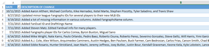
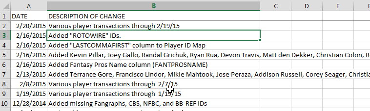
The “Change Log” tab of the Player ID Map will work the same way. Right-click and refresh the connection on that page to get an updated listing of the changes that have been made.
In the past you would have to come back to the site, download a new copy of the Excel file, and then paste it into your existing spreadsheets. Now you’ll just need to right click (or keep reading to see how you can have it update automatically) and update it!
The Links
The Player ID Map and Change Log are available in a variety of formats, depending on the goal you’re trying to accomplish.
This is a link to download the Player ID Map now containing a connection to an online source, so that when I add players to the list, they can easily be refreshed in your files.
This is a web page version of the Player ID Map. You can web query it into your Excel files or simply look at the list if you’re searching for a piece of information.
This link can be used to create a connection to an online CSV version of the Player ID Map that you can set up within Excel. We’ll take a closer look at how to do this in a set of instructions below.
This is a web page version of the Player ID Map Change Log. You can web query it into your Excel files or simply look at the list of changes to see what updates have recently been applied.
Similar to the CSV of the actual Player ID Map, this link can be used to create a connection to the change log within Excel. We’ll take a closer look at how to do this in a set of instructions below.
What If I Currently Have the Old Player ID Map in my File?
It’s great that the newly downloaded Player ID Map comes with the connection. But what about those who have the old version? Here’s a short set of instructions of how to establish this connection.
In this post I’ll show you how to add batter and pitcher handedness to your spreadsheets. To do this, we’ll have to learn two new Excel formulas we have not tackled yet.
I’ve avoided doing this for a long time… But there’s just no way around it now. It’s time to say goodbye to relying exclusively on VLOOKUP. Let’s put on our big boy pants and tackle VLOOKUP’s more flexible and powerful counterpart… INDEX and MATCH.
Sometimes VLOOKUP Can’t Get the Job Done
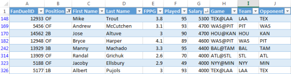
Take this scenario. You’ve started to build a DFS spreadsheet and you’ve imported FanDuel player salaries from a CSV file. Now you want to add player handedness (Lefty/Righty) as a column to your spreadsheet.FanDuel Salary Information
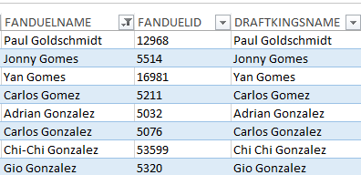
You are also aware of the Player ID Map and know that it’s an easy way to get handedness information on players.The Player ID Map contains information for batter and pitcher handedness, date of birth, team, position, and many player ID and naming systems.
You look at this data above and you think, “No problem!”. FanDuel ID is in both sets of data. How hard could this be? A simple VLOOKUP and we’re done.
But you quickly realize things are not that easy. You see, the VLOOKUP has a very restrictive assumption. If you are doing a VLOOKUP from the salary information into the Player ID Map, the Excel function assumes that “FanDuelID” will be the FIRST column in the Player ID Map.
And that’s NOT the case.
Let’s look at an example VLOOKUP formula:
=VLOOKUP([@FanDuelID],PLAYERIDMAP,10,FALSE)
In this formula we’ve told Excel to go look for the “FanDuelID” column in the “PLAYERIDMAP” table and give us back the value in the 10th column.
But “FanDuelID” is not the first column of the PLAYERIDMAP. It’s the 33rd (wow… the Player ID Map is getting to be quite large). So VLOOKUP will not work.
Other Weaknesses of VLOOKUP
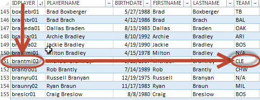
Not only is assuming the data you want to match is in the first column awfully restrictive, if you think about it, VLOOKUP also ties you to a left-to-right lookup. For example, if you’re trying to use Excel to VLOOKUP which team Michael Brantley plays for, his player ID must be in the first column of your data set and you are then forced in to looking only to the right.
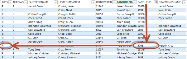
We want a formula that will allow our lookup to be in any column and then to look to the left! For example, go find Nelson Cruz’s FanDuelID and then look to the left a few columns and give me the side of the plate he bats from.
=VLOOKUP([@FanDuelID],PLAYERIDMAP,10,FALSE)
Going back to this example formula right above, the hard coding of a “10” in the formula to return the information in the 10th column is a flimsy approach, but that’s how many people are taught to write VLOOKUP formulas.
The flimsiness comes in if you decide to insert a column somewhere in the PLAYERIDMAP. If column 10 becomes column 11, Excel will not adjust its formula accordingly. Because you are likely building a spreadsheet that you’ll use all throughout the season, it seems highly likely you’ll want to add a new piece of information to your analysis. That inevitably means adding columns to bring that new information in. You don’t want to have to hunt through your formulas to figure out what the new column number in your VLOOKUP needs to be.
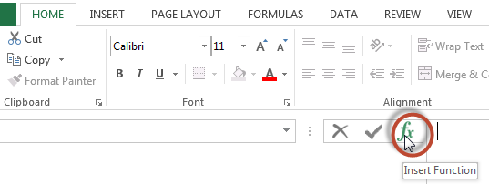
When I’m using a function I’m unfamiliar with, I will add it through the “Insert Function” button. I like doing this because Excel will then give you a search menu to find a formula. And after locating your function you’ll get a helpful wizard that breaks down all the inputs it needs.
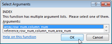
If you follow that approach to add the INDEX function, you’ll soon realize there are two versions of it.
I always use the first version, which allows us to locate a cell anywhere within a block of data and return the value from that cell. This function uses the following inputs:
INDEX(Array, Row_num, Column_num)
Array – The range of cells you are searching for a value in. This could be a table or a block of cells.
Row_num – The row within that array that the value is in. This should be a number representing the row.
Column_num – The column within the array that the value is in. Again, this should be a number representing the column (not the letter representation of the column).
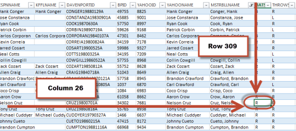
It may help to see a visual representation of the function. Assume we’re trying to find Nelson Cruz’s batting handedness. If we tell the index function to look in the PLAYERIDMAP (the “array”), in row 309 (“row_num”), and column 26 (column_num), it would return “R”.
We know the array to look in. And we can easily determine the column we want to look in. The challenge we now face is how to determine the row to look in… How do we easily determine that Nelson Cruz is listed on row 309. That’s where the “MATCH” function can help us.
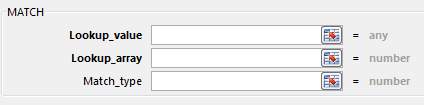
MATCH
The MATCH function will look for a specific value in a range of cells. The function will return a number representing where the matched item falls in the list.
Translating that into English, a realistic use for the function is to look in an entire column for a match. The function will start at the top of the column and proceed down until it locates the desired value. The function then returns where the item falls in the list, which happens to be the row the item is in.
The function uses these inputs:
MATCH(lookup_value, lookup_array, [match_type])
Lookup_value – This is the value you are hoping to match in the array (or column). For us, this will usually be a Player ID of some sort.
Lookup_array – This is the area you are searching for the match within. When using the MATCH function with the INDEX function, this will usually be a column of data.
Match_type – This is an optional input telling Excel some more details about the kind of match you are looking for. You can enter a 1, 0, or -1. Entering a 1 or -1 are forms of approximate matches and are useful if you are looking up numeric values. But we are typically looking to match strings (I consider a Player ID made up of all numbers to still be a string) of text.
This means we want exact matches only. Accordingly, I always use a 0 for this argument (even though it’s optional, leaving it blank tells Excel an approximate match is acceptable).
Combining INDEX and MATCH
As I alluded to before, the power of these two formulas comes when you combine (or nest) them together. Recall that the INDEX function looks like this:
INDEX(Array, Row_num, Column_num)
If we drop the MATCH function in place of the “Row_num” argument:
We now have a formula that is more flexible and powerful than a VLOOKUP! The combination of INDEX and MATCH can look for a value anywhere in a table of data and we are no longer tied to the first column and a right-only lookup.
Short and sweet update here… Columns for “FanDuelName”, “FanDuelID”, and “DraftKingsName” have been added to the Player ID Map (click to download the Excel file).
FANDUELNAME, FANDUELID, and DRAFTKINGSNAME columns have been added to the Player ID Map.
New to the site? Here are some past articles about how to use the Player ID Map in developing your spreadsheets (they focus on the season-long game, but the principles of using Player IDs or the map to account for differences in player names across sites still apply).
Please keep in mind that the Player ID Map is not intended to be all encompassing. I aim to keep all “fantasy relevant” players on the list. On choice days when a bench player or swing-man starting pitcher get the call, one might argue they become “fantasy relevant” to the daily game, but such players may not be included in the listing. I have to draw the line somewhere!
I’ve been exclusively focusing on web querying Fan Duel to this point. But what about Draft Kings? Is there a way to web query their salary information? Here’s an e-mail I recently got from a reader of the site…
Hey Tanner, I just got back from vacation and saw some of your recent posts. That looks great… but I play on Draft Kings. When I try to do those steps on that site, it doesn’t work. No player names. No salaries. Any ideas?
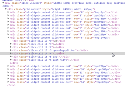
There is no <Table> element on the Draft Kings salary info.
I followed the same web querying steps we went through in this post, “How to Use Excel to Web Query DFS and Other Fantasy Baseball Data”, using FanDuel’s site this time. And sure enough, no matter what web querying option you use… No dice. If you do an investigation using the “Inspect element” option for your browser, I believe the technical reason the web query is unsuccessful is because the salary information is not coded as an HTML table.
So things aren’t going to be as easy as the web query. But due to a nice feature on Draft Kings, we can get very close. It’ll take just a few extra mouse clicks to get to the same place.
You see, even running a FanDuel web query isn’t seamless. You still have to log into your FanDuel account in your browser, locate a contest ID (URL), and type it into your Excel file to kick off the web query.
One Extra Step for Draft Kings
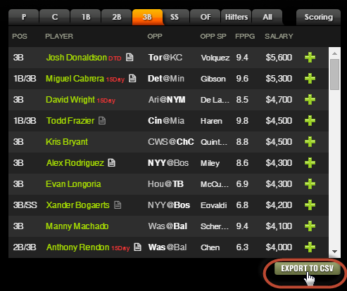
While Draft Kings salary info can’t be web queried, they do offer the ability to export all player information from a given contest into a nicely packaged CSV file. The link for a contest appears just below the player list you sort through to select players for your lineup.
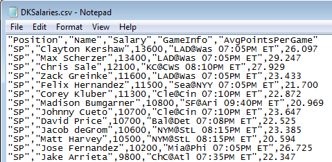
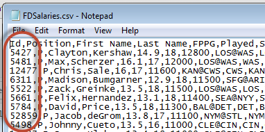
“CSV” stands for “comma separated values”. Many computer generated data export files have some kind of delimiter, or character, that breaks the data into columns. The CSV format specifically uses a comma to separate the values. Here’s what a CSV file looks like when opened outside of Excel:
That Looks Awful, How Do I Work With That File?
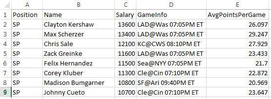
The CSV format does not look user-friendly when viewed outside of Excel. But fortunately, once you install Excel, it becomes the default program to open CSV files… And this format is so standardized, Excel is trained to clean up the data and put it in our friendly Excel format:
This Doesn’t Look as Efficient as a Web Query
Right about now you’re probably thinking something like this…
You mean to tell me each time I want to update my DFS baseball spreadsheet, I need to…
go Draft Kings,
find a contest to enter,
export the salary information,
open that CSV file,
copy the information,
and then paste it into my spreadsheet?
Not quite. Some of those things we have to do regardless. We can’t really automate the selection of the contest you want to enter. But we can have Excel automate steps four, five, and six (the process of getting the CSV data into a preexisting DFS spreadsheet.
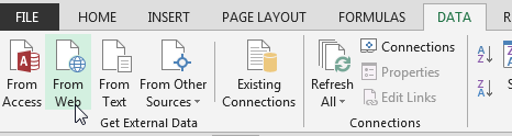
Excel Data From External Sources
You might remember in the previous web querying article that we used the “From Web” option to “Get External Data” into our Excel files.
Fortunately, Excel also has an external data option for “From Text” (and a CSV file is a text file) that works on the exact same principles of a web query.
Just like how the web query is set up to pull information from a very specific web URL, this text file link can be set up to pull information from a very specific file path.
So as long as we save and name our Draft Kings CSV file in the same place each time, the data can automatically pull in to our DFS Excel files each time we open it.
Step-By-Step Instructions
Step
Description
1.
Log into your Draft Kings account (unlike for a web query, you can use any browser you wish for this).
Once you’ve logged in, locate a contest you’d like to participate in and click the “ENTER>>” button.
2.
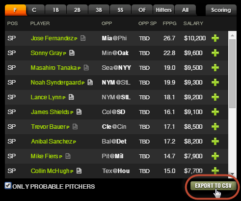
After the contest loads, click the “EXPORT TO CSV” button below the player salaries (located on the left half of the contest screen).
NOTE: It does not matter if you check or uncheck the “ONLY PROBABLE PITCHERS” box. The export always contains all pitchers.
3.
Depending on the browser you’re using and its settings, one of three things will likely happen at this point:
The CSV file will automatically download to your pre-specified download location
You’ll be prompted to name the CSV file and choose where to save the file
Or Excel may open and display the CSV file immediately
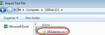
Regardless of what scenario you find yourself in, the main goal here is to save the CSV in a location where you want it to stay going forward. Maybe that’s your desktop or maybe you have a “Fantasy Baseball” or “DFS” folder on your computer. Save the CSV file in that long-term location.
So if it automatically downloaded to your “Downloads” folder, move it. If you’re being asked where to save the file, point it to the desired location. If Excel launched, perform a “Save As” to the desired folder. If you have the CSV file open, close it now.
4.
Open your DFS spreadsheet (you may want to make a backup before proceeding) or start a blank Excel file if you’re just beginning (don’t start in the CSV file!).
5.
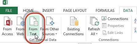
Go to the “Data” tab and click the “From Text” button.
6.
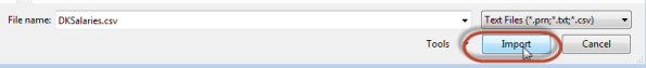
At this point Excel will prompt you to browse for the text file you want to import. Browse to and locate your CSV file.
Once you’ve located the file, select it and click the “Import” button.
7.
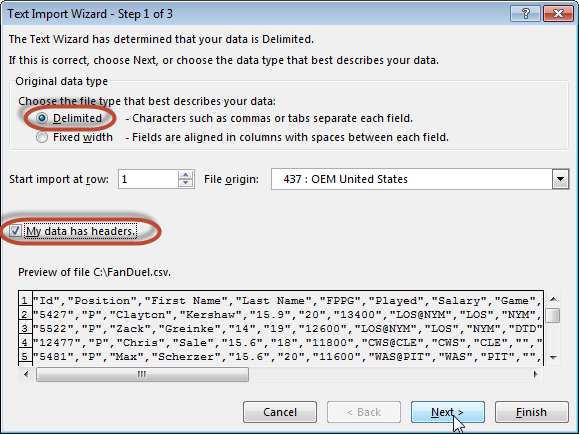
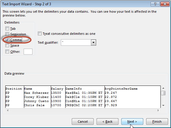
Excel’s “Text Import Wizard” will launch and ask which type of text file you’re importing. Remember that a CSV file is a special type of delimited text file that uses a comma to separate the values (a fixed width file doesn’t have a character (like a comma or semi-colon) separating the data, it would just have clearly visible spaces separating the data into columns). So choose the “Delimited” option.
Also check the “My data has headers” box and click “Next”.
On the next screen, choose the “Comma” delimiter option and uncheck any other options. You’ll get a preview of how the columns will be identified. Click “Next”.
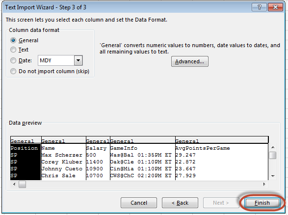
On the final screen of the Text Import Wizard you can likely just hit “Finish”. For future imports, if you have a column containing something you only want treated as text or a date, you can choose those options. But “General” is fine for our purposes.
8.
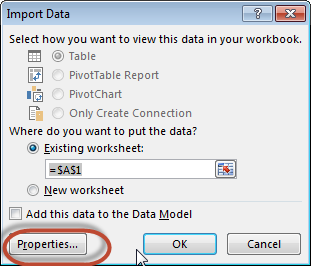
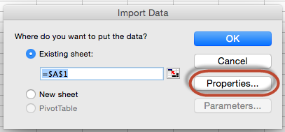
Once you click “Finish”, you’ll be prompted about where you want to import the CSV data to in the Excel file. If you are working in your pre-existing DFS spreadsheet, click on the tab you want the text to import to and use the “Existing Worksheet” option, or just choose the “New worksheet” radio button.
Don’t click OK yet! Click the “Properties” button.
9.
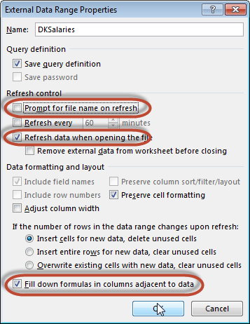
There are many available properties to adjust, but I’ll call out a few I feel the most strongly about changing:
Prompt for file name on refresh – If you plan to save the CSV file in the same location and with the same name each time, you should uncheck this option. If left checked, each time you refresh the connection to the CSV file you will need to browse to and select the file. Conversely, if you don’t want the restriction of having to name the file consistently and in the same spot, you may want this checked. But you’ll then need to browse and point to the new file each time you want to refresh the link.
Refresh data when opening the file – As you can probably guess, if you check this box, each time you open your DFS spreadsheet it will link to and import the text file information.
Fill down formulas in columns adjacent to data – We may not need this, but if we end up needing formulas next to the data being imported, I would recommend checking this box.
Click “Ok” to accept the settings changes.
Then click the next “OK” button on the “Import Data” window.
10.
That’s it! The next day, when you go to prepare for a new contest, simply repeat steps 1 through 3.
In doing so, be careful to name or save the CSV with the exact same name and in the exact same location as your Excel file is looking to.
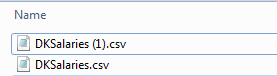
For instance, if you saved your first Draft Kings export as C:\Users\tanner.bell\Downloads\DKSalaries.csv, then make sure you save it there again the next day. If you have an older CSV already sitting in that location, the export will likely save as “DKSalaries (1).csv”. Not a problem. Just delete the older one and rename the new download to be just “DKSalaries.csv” (right-click on the file and choose “Rename”).
Web Query vs. CSV Import
I’m not sure which is superior or if there is even a clear winner. There is something elegant about the web query. And I really like how you can create a dynamic web query (I wish there were a way to do a dynamic text file link, but I can’t see a way to do that). But the web query is slow.
The text file import does require a couple of extra steps, in terms of naming the CSV file, but once that part is complete it’s essentially the same. The actual import of the data into Excel is much faster for the text file option (at times my web queries can take 30 seconds or more to complete).
For both options, Excel will seamlessly import the data and the rest of your Excel file can be built around this to automatically update based on the salary list.
Second Look at FanDuel
Having noticed this for Draft Kings, I took another look at FanDuel… Lo and behold, FanDuel has the same export option.
One key difference in the FanDuel CSV is that it has a unique file name associated with the contest ID.
So if you decide to go the CSV route for FanDuel, instead of using this unique name, rename/save the file with a generic name like “FDSalaries.csv”. If you also save the file in the same location each time, you would be able to link an Excel file to it repeatedly. At that point, just follow the setup instructions above and there is no difference in the setup of a FanDuel export and a Draft Kings export.
But Wait… What is that on the FanDuel Salaries List???
Oh my… This might be enough to convert me off the web query and to an exported CSV approach even for FanDuel (damn you Chris Youngs and Jose Ramirezes!).
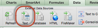
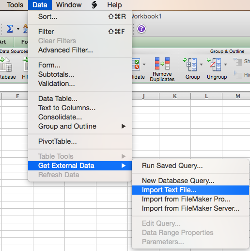
If you happen to be using Excel on a Mac, the menu location to start the import process is slightly different. You can find it on the “Data” tab.
Or you can also find it under the Data menu.
Once you find these menu options, the settings are the same as above (for the most part). Make sure to click on the “Properties” button to get options about when and how to refresh the import upon opening the Excel file.
How Is Your DFS Spreadsheet Coming Along
Do you have any neat features you’ve added? Struggling to get some kind of information added? Feel free to post a message below to share what you’ve done or let me know your struggles and maybe I can help.
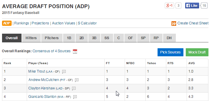
In this post I’ll show you how to link live average draft position information from the web into your draft spreadsheet. Every time you open your rankings file it will pull down updated ADP information. Bam!
How We’re Going To Do This
We will use a powerful feature of Excel called web querying to pull in the ADP information aggregated by FantasyPros.com (please note, I’m an affiliate of Fantasy Pros). The web query will suck up that table of ADP information and bring it directly into Excel for us to then VLOOKUP into our existing “Hitter Ranks” and “Pitcher Ranks” tabs.
Fantasy Pros has the best ADP information I’ve found on the web. They have the most sources in one place and it appears to be updated regularly.
Assumptions
I am assuming that you’ve followed my Standings Gain Points or Points-League Ranking series and are already starting with a spreadsheet that is based off one of those (you don’t have to have those exact spreadsheets, but something similar).
Excel Functions and Concepts Used in this Post
Web Query
As you can probably imagine, the power of the web query is that it automatically updates the data in your Excel file without you having to do ANYTHING after the initial setup.
Web queries are created from the “Data” tab on the Excel Ribbon, under the “Get External Data” icon grouping. There are several ways to get data from outside sources into Excel, we will be using the “From Web” button.
One “weakness” I have found in web queries is that they cannot work with “tables” in Excel. You cannot pull a web query in as the data of a table. If you’re a big follower of this site you know that’s a bit of an issue for me because I use tables all the time. Thankfully this doesn’t prevent us from doing things, I just point it out because you might wonder why I set things up the way I do in the instructions below.
Find
The FIND function searches within a specified cell for a string of text that you provide. If the FIND function locates the string, it will return the character position where the string starts at.
I know, you’re thinking “What the heck does that even mean?”. Here’s an example. Let’s say we have the text “Mike Trout (LAA)” in a cell and every player in our whole spreadsheet follows that format. If we want to pull out each player’s team we will need to start by figuring out where the team name starts in that cell. And we can’t just say it will always start at the 13th character each time when we have players like this hanging around MLB.
Instead we can use the FIND formula to intelligently determine where that opening parenthesis is for each player (it starts at 12 for Trout and 23 for Salty).
This formula requires two inputs:
FIND(Find_text, Within_text)
Find_text – This is the string of text you are searching for and keep in mind it is case-sensitive. You would wrap the string you are searching for in quotation marks. So in our example above, to look for the opening parenthesis you would enter “(” here. Or if you’re trying to be slightly more precise, you could enter ” (“, a space before the parenthesis.
Within_text – This is the text you want to search WITHIN. This can be a cell number.
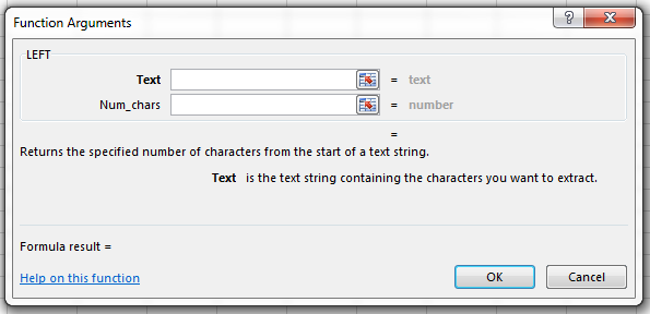
Left
The LEFT function gives you the leftmost number of characters in a text string. You also get to specify the number of characters to specify.
For example, if you have a text string of “Mike Trout (LAA)” and you ask for the 10 leftmost characters in that string, you would get “Mike Trout” back.
This formula requires two inputs:
LEFT(Text, Num_chars)
Text – This is the text string you want the leftmost characters from.
Num_chars – This is the number of characters you want from the string. This can be a hard entered number (e.g. 10) or it can be a formula itself that results in a number.
Combining Functions Together
We can do something pretty powerful by combining the FIND and LEFT functions together. I’ve been hinting at it with this “Mike Trout (LAA)” example. Recall from above that the LEFT function wants to know our text string (“Mike Trout (LAA)”) and the number of characters on the left to pull from that string.
Assume that cell B2 has a value of “Mike Trout (LAA)”. Instead of using this formula:
LEFT(B2, 10)
We can use this:
LEFT(B2, FIND(" (",B2)-1)
The FIND(" (",B2)-1 part of the formula returns a 10 (if you don’t subtract the one it returns an 11), and “Mike Trout” has 10 characters in it (including the space). By using this combination of functions we don’t have to type in a “10” for Mike Trout and a “21” for Saltalamacchia.
Important Prerequisite
Before you’re able to proceed with the instructions below you must make sure the PLAYERIDMAP in the file you’re working with was updated after February 21st, 2015. I added a column to the Player ID Map called “FANTPROSNAME” that is necessary for the steps below to work.
Instructions for updating your PLAYERIDMAP can be found here. Completing the update should only take five minutes or so.
Warning – The instructions below are likely only relevant if you are following some of my much older work. The Player ID Map has since been updated to allow much easier updating. If you’re looking for guidance relating to a spreadsheet you’ve built or purchased since 2015, you likely want to be looking here for guidance relating to the Player ID Map.
You’ve been following the site for a while. You’ve even created a spreadsheet to develop your own points league or SGP rankings. You’ve spent all this time building this spreadsheet but it’s getting to be a bit out of date. Players have been traded, rookies have been called up from the minors…
How do you update things? Do you have to rebuild your spreadsheets from scratch each season?
In this post I’ll show you how to quickly and easily update the Player ID Map in your spreadsheet so you can get updated MLB teams and have new players available to tie in to your projections.
Warning!
All we’re really doing here is downloading the new version of the Player ID Map and pasting it on top of our existing Player ID Map already in your ranking file. The key is that you have to be very particular about how you paste the new version in. If you’re not careful you will break all the existing formulas in your spreadsheet that reference the PLAYERIDMAP named table.
Read carefully!
Step-by-Step Instructions
Step
Description
1.
Open your existing rankings spreadsheet, the one in which you want the new Player ID Map information. Save a backup copy of the file, just in case something were to go wrong during this process.
Go to the PLAYERIDMAP tab.
2.
We will soon be pasting information onto this sheet so it is important to make sure all the data is currently showing.
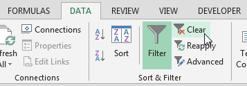
Click on Excel’s “Data” tab and then click the “Clear” button of the “Sort & Filter” icon grouping.
Once the download completes, open the file. If Excel is displaying any kind of warning message, enable your ability to edit the file (provided you trust this site).
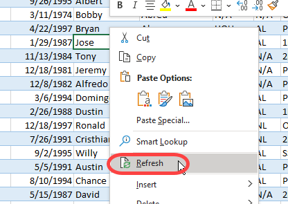
Now refresh the content to pull in any recently added players. Do this by right-clicking on a cell within the table (somewhere within the blue and white rows of data). Then choose the option to “Refresh.”
4.
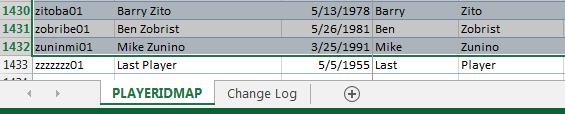
Place your mouse in cell A1 of the newly downloaded Player ID Map. Then hit the CTRL + SHIFT + End keys all at once. After you’ve done this release the keys. Then hit SHIFT + the up arrow key.
This set of key strokes should select the entire Player ID Map table and then deselect the “Last Player”.
Now hit CTRL + C to copy the selected data.
5.
Return to your customized rankings spreadsheet. Select cell A1 with your mouse and then paste the data you just copied over cell A1.
The reasoning behind this specific set of copying and pasting instruction is so that the existing table named “PLAYERIDMAP” in your rankings spreadsheet will not be renamed during this process. If you don’t deselect the “Last Player” before copying, the entire Player ID Map table will be renamed and it will break all existing VLOOKUP formulas you have looking for this information.
6.
That’s it!
Well, kind of. Any new players added to the PLAYERIDMAP will not yet be listed on your “Hitter Ranks” or “Pitcher Ranks” worksheets.
This is where you have a decision to make.
If you have taken notes next to players, entered keeper dollar values, or otherwise “hard entered” information that relates to a specific player, then you manually add the player IDs of “new” players to your “Hitter Ranks” or “Pitcher Ranks” tabs.
For example, simply go to the “Hitter Ranks” tab and type the player’s ID at the very bottom of the first column. When you hit enter the Excel table should grow to add your new player and all the other formulas should automatically copy down (another benefit of using Excel tables!).
If you’re not sure what players were added to the PLAYERIDMAP, you can look on the “CHANGE LOG” tab on the newly downloaded Player ID file to see a brief note of all the players added or updated recently.
I try to put brief descriptions of the players that have been added so you can manually add to your “Hitter Ranks” or “Pitcher Ranks” sheets, if necessary.
7.
If you have not edited dollar values or added player notes, you can copy and paste the hitter IDs onto the “Hitter Ranks” sheet and the pitcher IDs on to the “Pitcher Ranks” sheet.
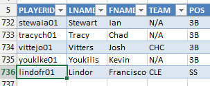
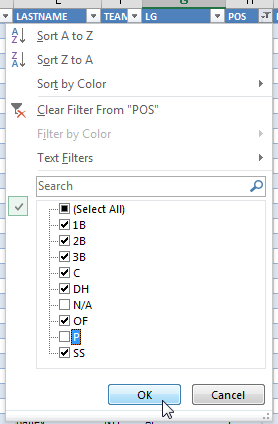
To do this, go to the PLAYERIDMAP tab in your spreadsheet and apply a filter to only show hitters. On the “POS” column filter, uncheck the “N/A” (if there are any) and “P” check boxes. This will only display the hitters.
Then select cell the first cell below the header in column A and hit the SHIFT + CTRL + Down Arrow Key. Copy this information and go to your “Hitter Ranks” tab and paste it into the first cell below the header in column A there.
After you do this all the other information on the tab should update immediately.
No go back to the PLAYERIDMAP tab and adjust the filter to only show pitchers and repeat the process by pasting those players onto the “Pitcher Ranks” tab.
Now you’re done!
Have Any Questions?
Please leave a comment on this post.
I have to do this quite frequently to keep all the spreadsheets I maintain for the site up-to-date, but this is probably something you’ll only need to do a few times a year. Maybe after the season ends, to get all the new players I’ve added during the season, late February, to get all the players that have changed teams, and once during the season, if you’re doing in-season rankings.
Want More Tips Like This
Make sure to follow me on Twitter, that’s the best place to hear about new posts and updates at the site.
After over a year of working on this and getting feedback from a very helpful group of SFBB readers, the “Projection Aggregator” Excel file is finally ready!
The Projection Aggregator is an easy to use Excel spreadsheet that can combine (or average) up to three different projection sets to give you the best possible set of projections to use for the upcoming season. You can use just about any well known projection source you have at your disposal. Download your favorite projections, fill out some settings, and you’re done.
No complicated formulas. No VLOOKUPs. Just download your projections, bring them in to the Aggregator, and you’ll have better projections in minutes. Click here to find out more.
When you’re building a rankings spreadsheet, why don’t you just build the calculations right on the projection tab?
Why do you even use this ridiculous Player ID map? There’s so much useless information on that thing.
Have You Ever Wondered These Things?
I have to say that I haven’t had anyone ask these questions, but I feel the need to address the questions nonetheless. I don’t mean for them to be overly complicated, but there’s a good chance that the spreadsheets I design can be overwhelming. So let’s take a closer look at the reasoning behind things.
There Is More Than One Way To Skin a Cat
I don’t think it’s much of a stretch to say that spreadsheet design is a form or art. There are many different ways to get to the same end goal. I’m always looking for new ideas and methods to add to my Excel work, and I’m certain there are more efficient and better ways to design things I have done.
With that said, I believe the principles I’m about to talk about are universal. Whether you like the way I’ve designed things or if you prefer to do things a different way, using these concepts should help you out in the long run.
Why Do Your Spreadsheets Have So Many Tabs?
There are two main reasons for this:
I want all of my spreadsheets to be reusable.
I try to set things up so you only have to enter a piece of information one time.
Reusable Spreadsheets
We’ll take a close look at reusable design in a moment, but think about the different tabs/worksheets I use. Raw projections, player information, replacement level information, and calculations all on separate worksheets.
By setting these up on distinct areas of a spreadsheet it allows you to easily update one of those components without screwing up the whole model. Have new projection info? Just replace the data on the projection tab. Have a new Player ID Map? Just copy it over top of the existing one.
This setup makes it much easier for your work to be updated during the season and into future seasons.
Entering Information Only Once
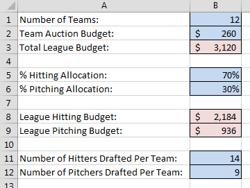
If you’ve read my book on calculating dollar values and in-draft inflation, you’ll recall that we added a “Settings” tab to the rankings spreadsheet. On that tab we color-coded blue cells to indicate input cells.
These are just basic settings about the league, but by separating them out onto the “Settings” tab you only have to type the information one time. If we didn’t do this, we would have to embed this information into our calculations for both the hitting and pitching rankings.
Everything is also formula-driven, so if a 13th team is added next year, or if team salary caps increase, or if you want to try a 65% hitting allocation, you can easily change those inputs and all calculations for hitters and pitchers update automatically.
If we didn’t have things set up this way you would have to search deep inside complex formulas on the hitter tab and edit these inputs. And then you’d have to go do the same thing on the pitcher rankings.
And if you’re in more than one league you can set your rankings up for one league, just change the few settings different between the leagues, and you’ll easily have rankings tailored to each league you play in.
Why Don’t You Just Build Your Calculations Right on the Projections Tab?
Whether you’ve downloaded projections from another website or you’ve created your own, it might seem like I’m over-complicating things by having the projections on one tab and then using formulas to pull the projections to a whole other worksheet where I then calculate rankings, SGP, and dollar values.
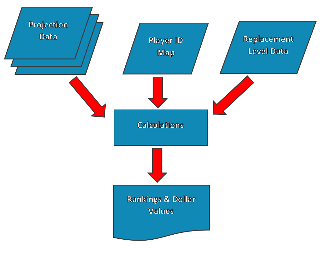
If I were to use this spreadsheet one time, I would agree with this line of thinking. But take a look at this image.
This is a very primitive flow-charting model of a rankings spreadsheet. You have a few sets of raw data as inputs (the blue rhombuses, or is it rhombi?) – the projections, the Player ID Map, and replacement level data. Continue reading “Designing Reusable Fantasy Baseball Spreadsheets”
We use cookies to ensure that we give you the best experience on our website. If you continue to use this site we will assume that you are happy with it.
 If you have Excel 2013 and you’ve downloaded the “new” version of the Player ID Map, you can right click anywhere in that tab of the spreadsheet and choose to “Refresh” the connection. Excel will seamless download the new updates to your file.
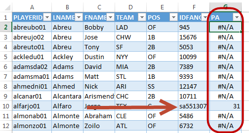

 You might remember in the previous web querying article that we used the “From Web” option to “Get External Data” into our Excel files.


 Copy this information and go to your “Hitter Ranks” tab and paste it into the first cell below the header in column A there.