I’ve been exclusively focusing on web querying Fan Duel to this point. But what about Draft Kings? Is there a way to web query their salary information? Here’s an e-mail I recently got from a reader of the site…
Hey Tanner, I just got back from vacation and saw some of your recent posts. That looks great… but I play on Draft Kings. When I try to do those steps on that site, it doesn’t work. No player names. No salaries. Any ideas?
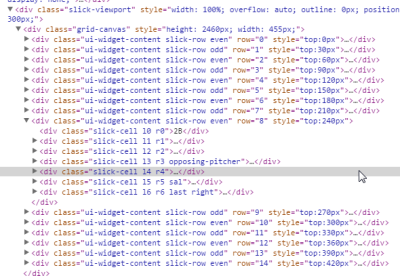
I followed the same web querying steps we went through in this post, “How to Use Excel to Web Query DFS and Other Fantasy Baseball Data”, using FanDuel’s site this time. And sure enough, no matter what web querying option you use… No dice. If you do an investigation using the “Inspect element” option for your browser, I believe the technical reason the web query is unsuccessful is because the salary information is not coded as an HTML table.
So things aren’t going to be as easy as the web query. But due to a nice feature on Draft Kings, we can get very close. It’ll take just a few extra mouse clicks to get to the same place.
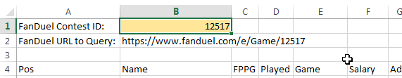
You see, even running a FanDuel web query isn’t seamless. You still have to log into your FanDuel account in your browser, locate a contest ID (URL), and type it into your Excel file to kick off the web query.
One Extra Step for Draft Kings
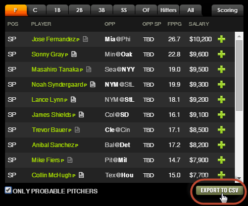
While Draft Kings salary info can’t be web queried, they do offer the ability to export all player information from a given contest into a nicely packaged CSV file. The link for a contest appears just below the player list you sort through to select players for your lineup.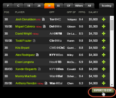
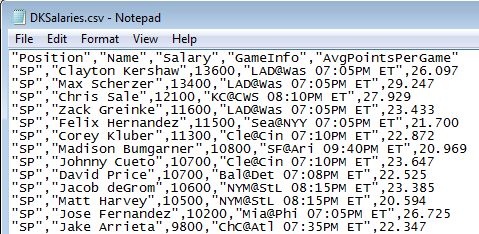
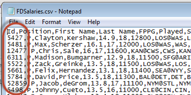
“CSV” stands for “comma separated values”. Many computer generated data export files have some kind of delimiter, or character, that breaks the data into columns. The CSV format specifically uses a comma to separate the values. Here’s what a CSV file looks like when opened outside of Excel:
That Looks Awful, How Do I Work With That File?
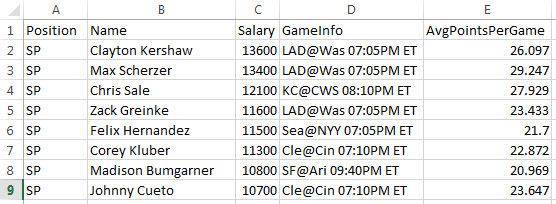
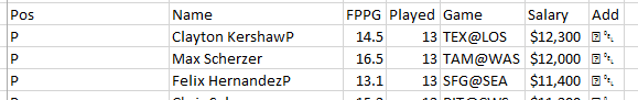
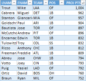
The CSV format does not look user-friendly when viewed outside of Excel. But fortunately, once you install Excel, it becomes the default program to open CSV files… And this format is so standardized, Excel is trained to clean up the data and put it in our friendly Excel format:
This Doesn’t Look as Efficient as a Web Query
Right about now you’re probably thinking something like this…
You mean to tell me each time I want to update my DFS baseball spreadsheet, I need to…
- go Draft Kings,
- find a contest to enter,
- export the salary information,
- open that CSV file,
- copy the information,
- and then paste it into my spreadsheet?
Not quite. Some of those things we have to do regardless. We can’t really automate the selection of the contest you want to enter. But we can have Excel automate steps four, five, and six (the process of getting the CSV data into a preexisting DFS spreadsheet.
Excel Data From External Sources
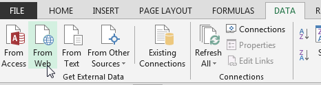
 You might remember in the previous web querying article that we used the “From Web” option to “Get External Data” into our Excel files.
Fortunately, Excel also has an external data option for “From Text” (and a CSV file is a text file) that works on the exact same principles of a web query.
Just like how the web query is set up to pull information from a very specific web URL, this text file link can be set up to pull information from a very specific file path.
So as long as we save and name our Draft Kings CSV file in the same place each time, the data can automatically pull in to our DFS Excel files each time we open it.
Step-By-Step Instructions
| Step | Description |
|---|---|
| 1. | Log into your Draft Kings account (unlike for a web query, you can use any browser you wish for this).
Once you’ve logged in, locate a contest you’d like to participate in and click the “ENTER>>” button. |
| 2. | After the contest loads, click the “EXPORT TO CSV” button below the player salaries (located on the left half of the contest screen).
NOTE: It does not matter if you check or uncheck the “ONLY PROBABLE PITCHERS” box. The export always contains all pitchers. |
| 3. | Depending on the browser you’re using and its settings, one of three things will likely happen at this point:
Regardless of what scenario you find yourself in, the main goal here is to save the CSV in a location where you want it to stay going forward. Maybe that’s your desktop or maybe you have a “Fantasy Baseball” or “DFS” folder on your computer. Save the CSV file in that long-term location. So if it automatically downloaded to your “Downloads” folder, move it. If you’re being asked where to save the file, point it to the desired location. If Excel launched, perform a “Save As” to the desired folder. If you have the CSV file open, close it now. |
| 4. | Open your DFS spreadsheet (you may want to make a backup before proceeding) or start a blank Excel file if you’re just beginning (don’t start in the CSV file!). |
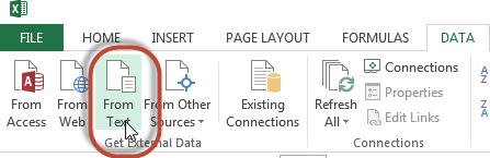
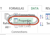
| 5. | Go to the “Data” tab and click the “From Text” button. |
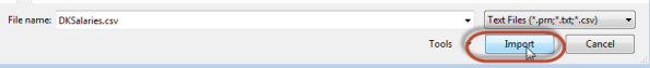
| 6. | At this point Excel will prompt you to browse for the text file you want to import. Browse to and locate your CSV file.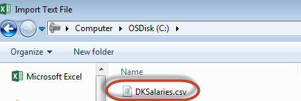
Once you’ve located the file, select it and click the “Import” button. |
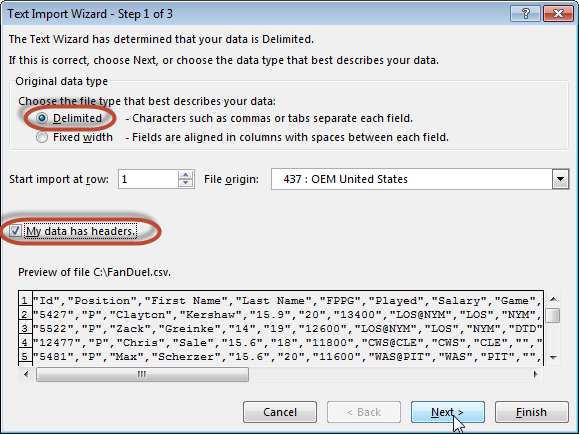
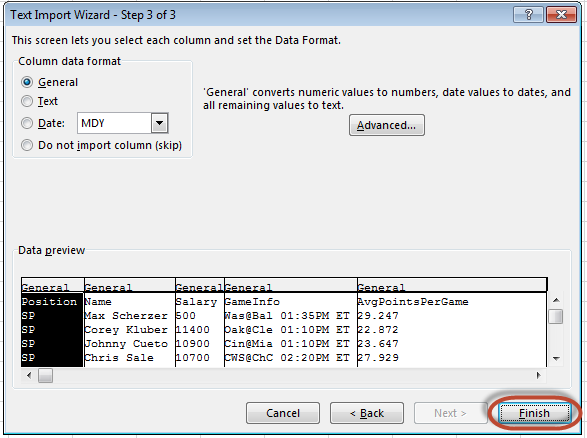
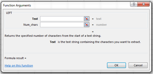
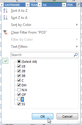
| 7. | Excel’s “Text Import Wizard” will launch and ask which type of text file you’re importing. Remember that a CSV file is a special type of delimited text file that uses a comma to separate the values (a fixed width file doesn’t have a character (like a comma or semi-colon) separating the data, it would just have clearly visible spaces separating the data into columns). So choose the “Delimited” option.
Also check the “My data has headers” box and click “Next”.
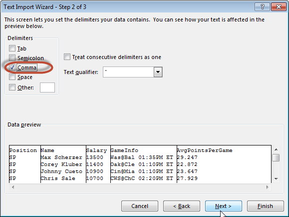
On the next screen, choose the “Comma” delimiter option and uncheck any other options. You’ll get a preview of how the columns will be identified. Click “Next”. On the final screen of the Text Import Wizard you can likely just hit “Finish”. For future imports, if you have a column containing something you only want treated as text or a date, you can choose those options. But “General” is fine for our purposes.
|
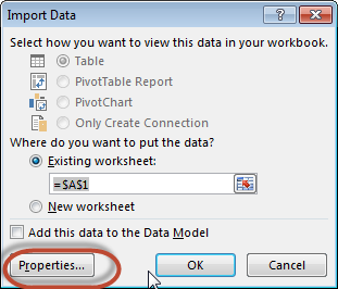
| 8. | Once you click “Finish”, you’ll be prompted about where you want to import the CSV data to in the Excel file. If you are working in your pre-existing DFS spreadsheet, click on the tab you want the text to import to and use the “Existing Worksheet” option, or just choose the “New worksheet” radio button.
Don’t click OK yet! Click the “Properties” button.
|
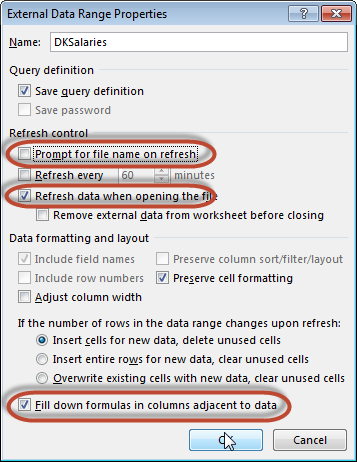
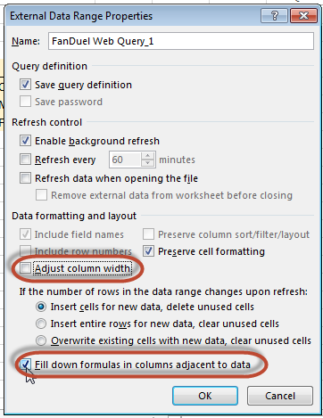
| 9. | There are many available properties to adjust, but I’ll call out a few I feel the most strongly about changing:
Prompt for file name on refresh – If you plan to save the CSV file in the same location and with the same name each time, you should uncheck this option. If left checked, each time you refresh the connection to the CSV file you will need to browse to and select the file. Conversely, if you don’t want the restriction of having to name the file consistently and in the same spot, you may want this checked. But you’ll then need to browse and point to the new file each time you want to refresh the link. Refresh data when opening the file – As you can probably guess, if you check this box, each time you open your DFS spreadsheet it will link to and import the text file information. Fill down formulas in columns adjacent to data – We may not need this, but if we end up needing formulas next to the data being imported, I would recommend checking this box.
Click “Ok” to accept the settings changes. Then click the next “OK” button on the “Import Data” window. |
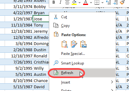
| 10. | That’s it! The next day, when you go to prepare for a new contest, simply repeat steps 1 through 3.
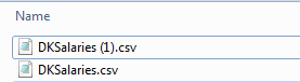
In doing so, be careful to name or save the CSV with the exact same name and in the exact same location as your Excel file is looking to. For instance, if you saved your first Draft Kings export as C:\Users\tanner.bell\Downloads\DKSalaries.csv, then make sure you save it there again the next day. If you have an older CSV already sitting in that location, the export will likely save as “DKSalaries (1).csv”. Not a problem. Just delete the older one and rename the new download to be just “DKSalaries.csv” (right-click on the file and choose “Rename”). |

Web Query vs. CSV Import
I’m not sure which is superior or if there is even a clear winner. There is something elegant about the web query. And I really like how you can create a dynamic web query (I wish there were a way to do a dynamic text file link, but I can’t see a way to do that). But the web query is slow.
The text file import does require a couple of extra steps, in terms of naming the CSV file, but once that part is complete it’s essentially the same. The actual import of the data into Excel is much faster for the text file option (at times my web queries can take 30 seconds or more to complete).
For both options, Excel will seamlessly import the data and the rest of your Excel file can be built around this to automatically update based on the salary list.
Second Look at FanDuel
Having noticed this for Draft Kings, I took another look at FanDuel… Lo and behold, FanDuel has the same export option.

One key difference in the FanDuel CSV is that it has a unique file name associated with the contest ID. ![]()
So if you decide to go the CSV route for FanDuel, instead of using this unique name, rename/save the file with a generic name like “FDSalaries.csv”. If you also save the file in the same location each time, you would be able to link an Excel file to it repeatedly. At that point, just follow the setup instructions above and there is no difference in the setup of a FanDuel export and a Draft Kings export.
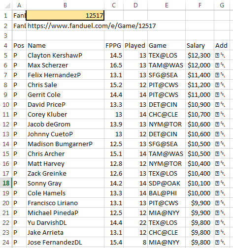
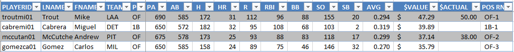
But Wait… What is that on the FanDuel Salaries List???
Oh my… This might be enough to convert me off the web query and to an exported CSV approach even for FanDuel (damn you Chris Youngs and Jose Ramirezes!).
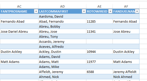
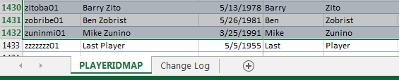
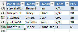
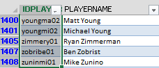
Player IDs (don’t know what a Player ID is?)… FanDuel player IDs, coming soon to a Player ID Map near you.
Doing This in Excel For Mac 2011
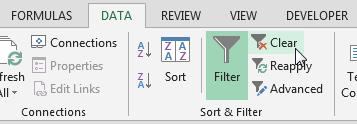
If you happen to be using Excel on a Mac, the menu location to start the import process is slightly different. You can find it on the “Data” tab. 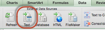
Or you can also find it under the Data menu.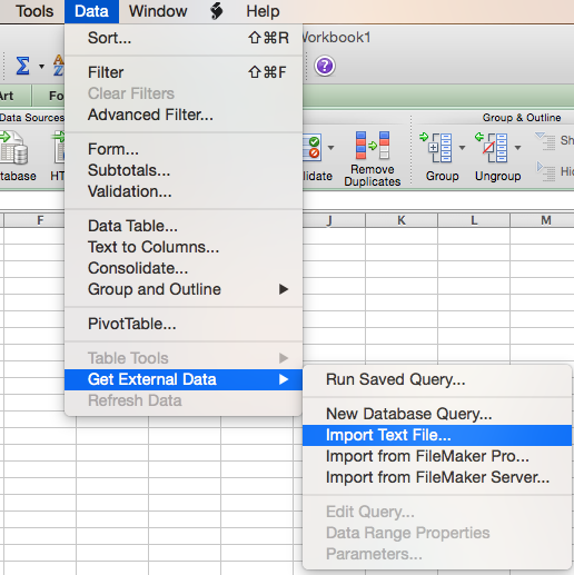
Once you find these menu options, the settings are the same as above (for the most part). Make sure to click on the “Properties” button to get options about when and how to refresh the import upon opening the Excel file. 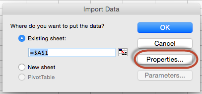
How Is Your DFS Spreadsheet Coming Along
Do you have any neat features you’ve added? Struggling to get some kind of information added? Feel free to post a message below to share what you’ve done or let me know your struggles and maybe I can help.
Stay smart.
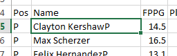
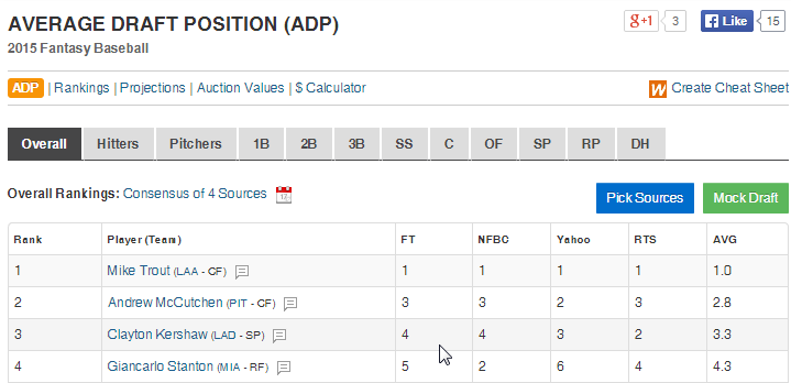


 Copy this information and go to your “Hitter Ranks” tab and paste it into the first cell below the header in column A there.
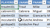

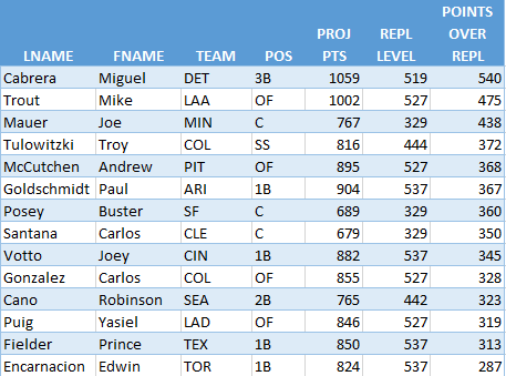

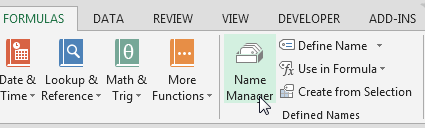
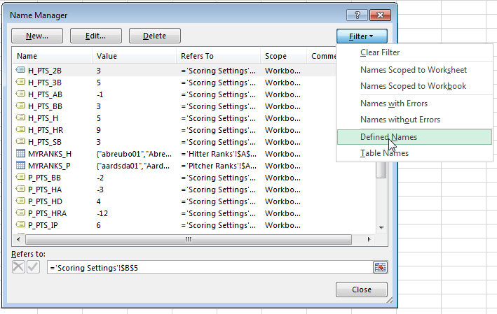
 To refresh your memory and to see the complete list of named cells, access the “Formulas” tab of the Ribbon and then click the “Name Manager” button.